

If you want to add up numbers based on a condition, Excel gives you two functions that look almost identical, SUMIF and SUMIFS.
And it’s not always obvious which one you should pick.
The short version is that SUMIF handles one condition and SUMIFS handles one or more.
But there are a few less obvious differences too, and some of them can quietly give you the wrong total.
In this article, I’ll show you how SUMIF and SUMIFS differ, with examples, the edge cases that trip people up, and a few things SUMIFS can do that SUMIF can’t.
Follow along with the example file
SUMIF vs SUMIFS Examples.xlsx
SUMIF vs SUMIFS: The Quick Answer
Here is how the two functions compare:
| SUMIF | SUMIFS | |
|---|---|---|
| Number of conditions | One | Up to 127 |
| Syntax | =SUMIF(range,criteria,[sum_range]) | =SUMIFS(sum_range,criteria_range1,criteria1,...) |
| Where the sum range goes | Last | First |
| Is the sum range optional? | Yes | No |
| Two AND conditions on the same column (like a date range) | No, needs two SUMIFs | Yes, in one formula |
| Ranges of different sizes | Quietly resizes the sum range | Returns #VALUE! |
In most cases, SUMIFS is the safer one to use.
It does everything SUMIF does, it lets you add a second condition later without rewriting the formula, and it throws an error instead of quietly using the wrong cells.
SUMIF is still perfectly fine for a quick one-condition total, especially when the numbers you’re checking are the same numbers you’re adding.
Here is the same task done with each function. All of these formulas use the example dataset, and each one is explained in its own section below:
| Task | SUMIF | SUMIFS |
|---|---|---|
| London total | =SUMIF(B2:B13,"London",D2:D13) | =SUMIFS(D2:D13,B2:B13,"London") |
| Sales over $300 | =SUMIF(D2:D13,">300") | =SUMIFS(D2:D13,D2:D13,">300") |
| London AND Fiction | =SUMIF(E2:E13,"London-Fiction",D2:D13) (needs a helper column in E) | =SUMIFS(D2:D13,B2:B13,"London",C2:C13,"Fiction") |
| Between two dates (F2 to G2) | =SUMIF(A2:A13,">="&F2,D2:D13)-SUMIF(A2:A13,">"&G2,D2:D13) | =SUMIFS(D2:D13,A2:A13,">="&F2,A2:A13,"<="&G2) |
| London OR Paris | =SUM(SUMIF(B2:B13,{"London","Paris"},D2:D13)) | =SUM(SUMIFS(D2:D13,B2:B13,{"London","Paris"})) |
The criteria rules are identical in both, so wildcard characters, comparison operators like “<>” (not equal to), and cell references work the same way.
Every example below uses the same dataset of book sales from a store with branches in London, Tokyo, and Paris.
The Syntax Difference: The Arguments Are Flipped
The biggest practical difference between SUMIF and SUMIFS is the order of the arguments.
Here is the syntax of both:
=SUMIF(range,criteria,[sum_range])
=SUMIFS(sum_range,criteria_range1,criteria1,[criteria_range2,criteria2],...)
In SUMIF, the range you want to add comes last. In SUMIFS, it comes first. Let me show you what this looks like with the same calculation.
Below is the dataset, with the date in column A, the city in column B, the genre in column C, and the sales amount in column D. I want the total sales for London.
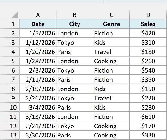
Here is the SUMIF formula:
=SUMIF(B2:B13,"London",D2:D13)
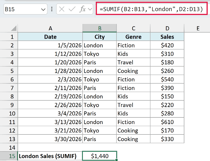
And here is the SUMIFS formula that gives the same result:
=SUMIFS(D2:D13,B2:B13,"London")
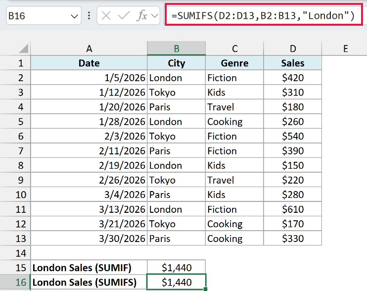
Both formulas return $1,440.
In SUMIF, I first tell Excel where to look (B2:B13), then what to look for (“London”), and finally what to add (D2:D13).
In SUMIFS, I start with what to add (D2:D13) and then give it the range and condition pair.
Important: If you switch a SUMIF to SUMIFS by just adding an “S”, the ranges end up in the wrong slots. Move the sum range to the front.
SUMIF Can Skip the Sum Range, SUMIFS Can’t
In SUMIF, the sum range is optional. If you leave it out, SUMIF adds the same cells it checks.
This comes in handy when the condition is on the numbers themselves, like adding up only the large sales.
Below is the same dataset. This time, I want the total of all sales that are more than $300.
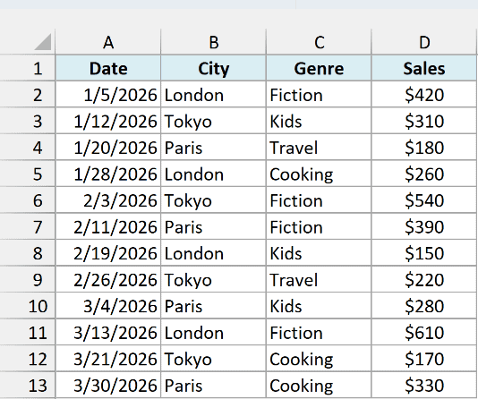
Here is the SUMIF formula:
=SUMIF(D2:D13,">300")
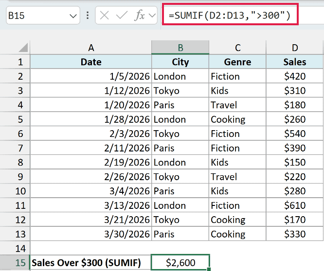
Since there’s no third argument, SUMIF checks D2:D13 against “>300” and adds the matching cells from the same range. This gives $2,600.
SUMIFS has no optional sum range, so you have to give it the same range twice:
=SUMIFS(D2:D13,D2:D13,">300")
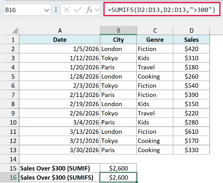
The first D2:D13 is the range to add, and the second one is the range to check. The result is the same $2,600.
Sum With Multiple Criteria: SUMIF Needs a Helper Column
This is the difference most people know about. SUMIF can check only one condition, while SUMIFS can check up to 127 of them.
So can you use SUMIF with two criteria? Not directly. But you can get there with a helper column, and comparing the two approaches shows why SUMIFS exists.
Below is the same dataset. I want the total sales of Fiction books in London, which means two conditions, one on the city and one on the genre.
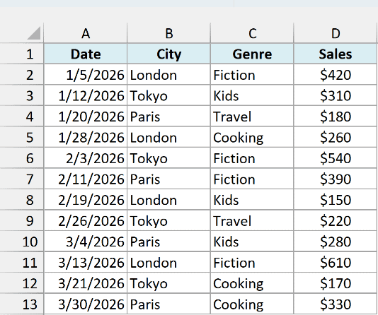
To make this work with SUMIF, I first need a helper column that joins the city and genre into one value. Here is the formula I entered in cell E2:
=B2:B13&"-"&C2:C13
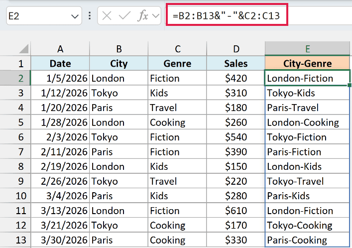
The formula spills down the column automatically, giving values like London-Fiction and Tokyo-Kids. Now the two conditions are one condition, which SUMIF can handle.
Pro Tip: In Excel 2019 or earlier, enter =B2&”-“&C2 in cell E2 and copy it down the column instead.
Here is the SUMIF formula:
=SUMIF(E2:E13,"London-Fiction",D2:D13)
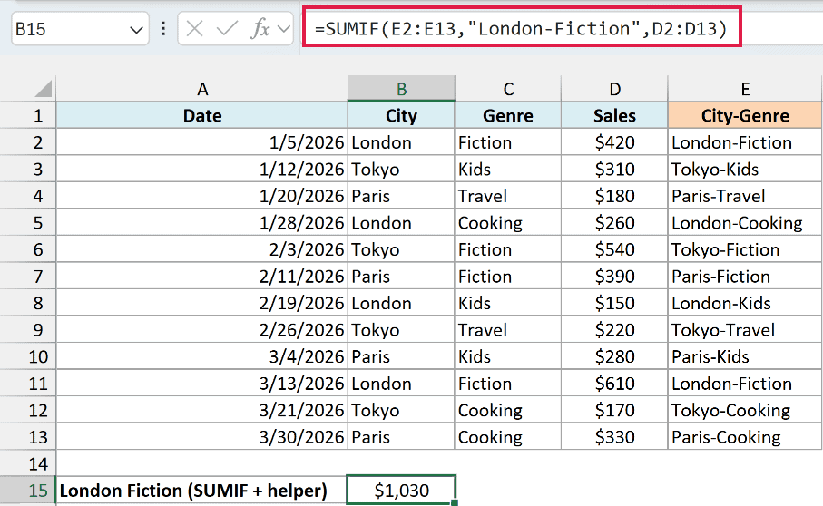
This gives $1,030, the total of the two London Fiction sales.
Now here is the SUMIFS formula that does the same thing without any helper column:
=SUMIFS(D2:D13,B2:B13,"London",C2:C13,"Fiction")
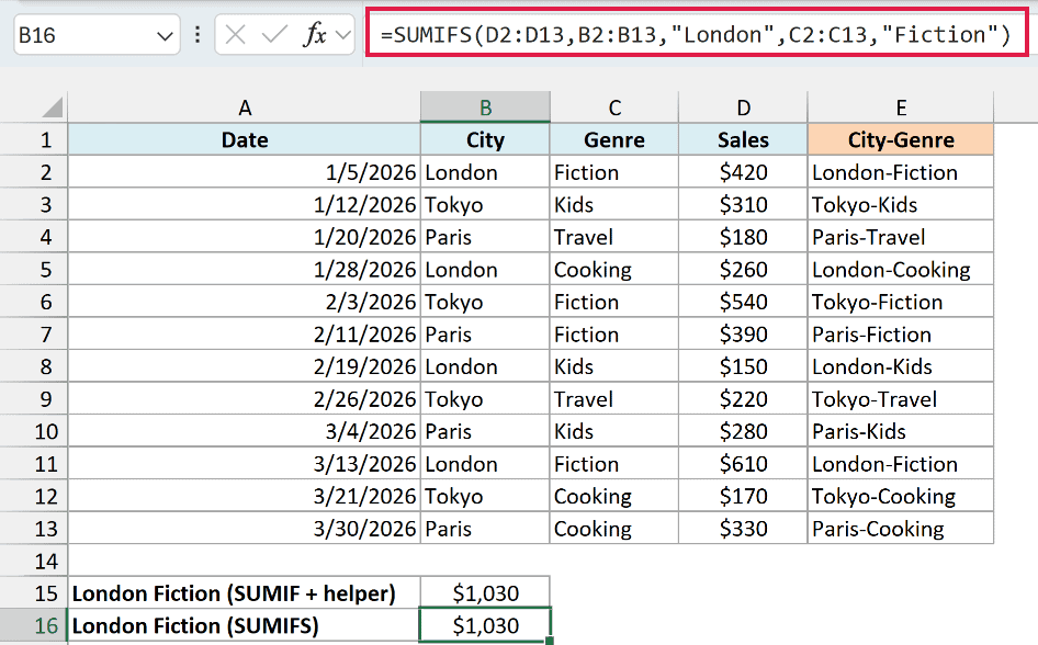
It gives the same $1,030.
SUMIFS adds a row only when every condition is true for that row. The first pair (B2:B13 and “London”) keeps only the London rows.
The second pair (C2:C13 and “Fiction”) keeps only the Fiction rows among those. Only the two rows that match both get added.
The helper column works, but it adds an extra column to your data, and a third condition would mean rebuilding it. With SUMIFS, you just add another range and condition pair.
Sum Between Two Dates: One SUMIFS vs Two SUMIFs
This one is less obvious.
SUMIFS lets you put two conditions on the same column, which is exactly what you need to sum between two dates.
Below is the same dataset, with a start date in cell F2 (2/1/2026) and an end date in cell G2 (3/15/2026). I want the total sales between these two dates.
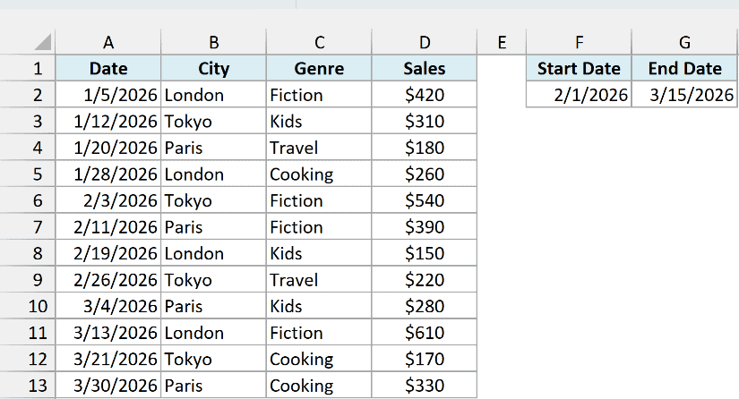
Here is the SUMIFS formula:
=SUMIFS(D2:D13,A2:A13,">="&F2,A2:A13,"<="&G2)
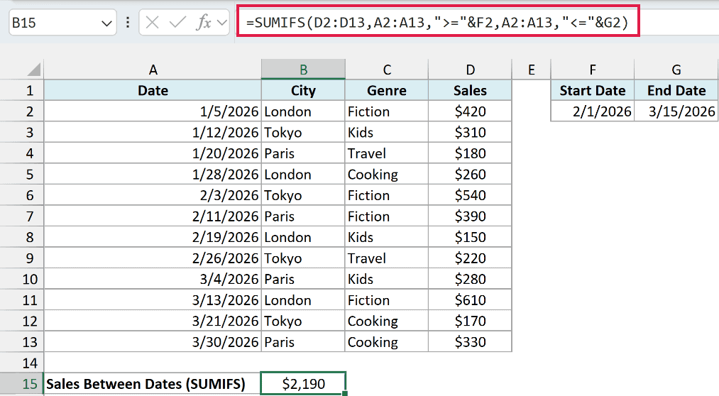
This gives $2,190.
I’ve used the date column (A2:A13) twice. The first condition keeps dates on or after the start date, and the second keeps dates on or before the end date.
The & joins the operator with the date in the cell, so “>=”&F2 becomes “on or after 2/1/2026”.
With SUMIF, you can’t check two conditions at once. So you need to add everything from the start date onward, then subtract everything after the end date:
=SUMIF(A2:A13,">="&F2,D2:D13)-SUMIF(A2:A13,">"&G2,D2:D13)
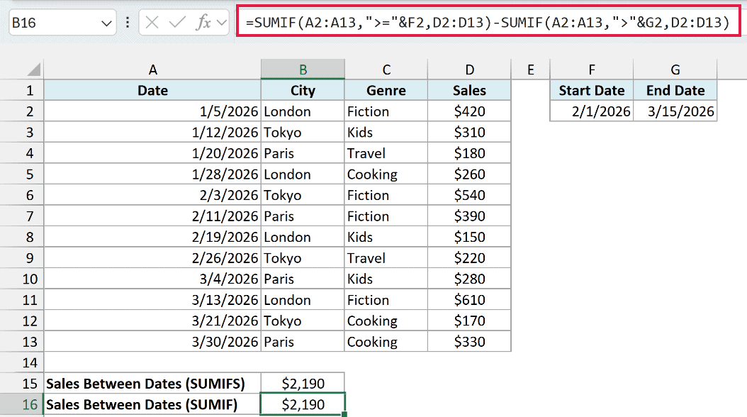
It gives the same $2,190, but it’s longer and easier to get wrong.
For example, if the end date were 3/13/2026, using “>=” instead of “>” in the second SUMIF would wrongly drop the $610 sale made on that day.
Follow along with the example file
SUMIF vs SUMIFS Examples.xlsx
What Happens When the Ranges Aren’t the Same Size
This is an edge case where the two functions behave completely differently.
SUMIF doesn’t care if the sum range is a different size. It starts at the first cell of the sum range and quietly stretches it to match the criteria range.
SUMIFS refuses and returns an error.
Below is the same dataset. I want the total sales for London again, but this time I’ve given each function only one cell (D2) as the sum range.
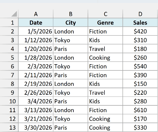
Here is the SUMIF formula:
=SUMIF(B2:B13,"London",D2)
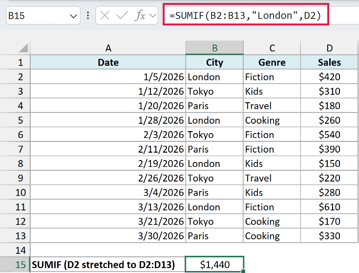
This still returns $1,440, the correct London total. Since the criteria range B2:B13 is 12 cells tall, SUMIF treats D2 as the start of a 12-cell range (D2:D13).
You’ll sometimes see this shortcut in older workbooks. It works, but Microsoft notes that it can slow the workbook down, and it hides what the formula is really adding.
Now here is the same thing with SUMIFS:
=SUMIFS(D2,B2:B13,"London")
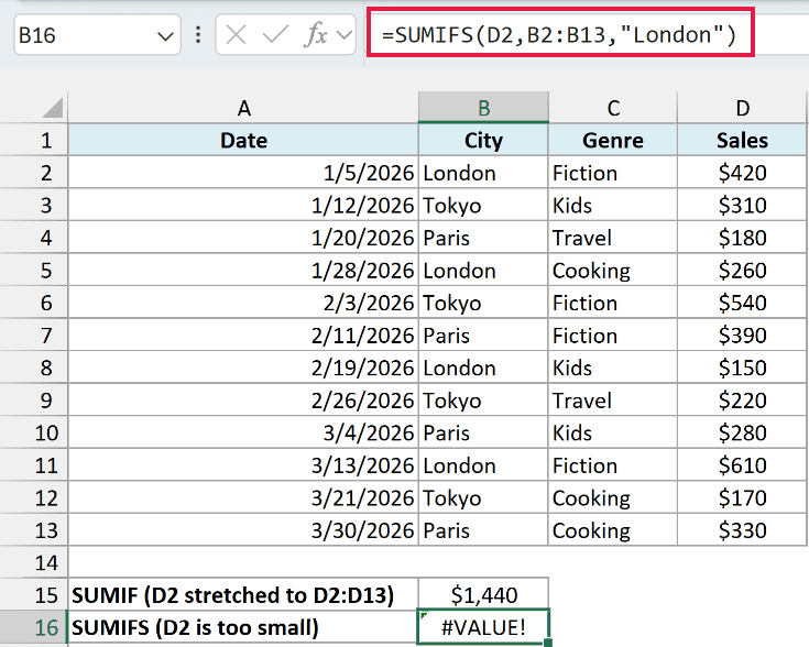
This returns a #VALUE! error, because in SUMIFS every criteria range must be the same size and shape as the sum range. The fix is to make the ranges match (D2:D13).
This is one more reason SUMIFS is the safer default. A loud error is easier to fix than a formula that silently adds a range you didn’t mean to select.
Important: Neither function catches shifted ranges. SUMIFS(D1:D12,B2:B13,”London”) gives $850 instead of $1,440 with no error, so make sure your ranges start on the same row.
Sum With OR Logic (The Same-Column Trap)
Multiple conditions in SUMIFS always work as AND. A row gets added only when all conditions are true.
This trips people up when they want an OR, like the total sales for London or Paris.
Below is the same dataset. I want the combined sales of the London and Paris branches.
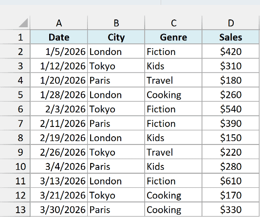
A lot of people try this first:
=SUMIFS(D2:D13,B2:B13,"London",B2:B13,"Paris")
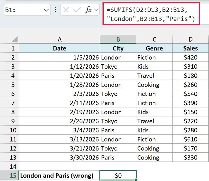
This returns $0. The formula asks for rows where the city is London and also Paris at the same time, and no cell can be both.
Here is the formula that does it correctly:
=SUM(SUMIFS(D2:D13,B2:B13,{"London","Paris"}))
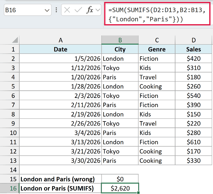
This gives $2,620.
The curly brackets hold a list of criteria, so SUMIFS runs once for London ($1,440) and once for Paris ($1,180). SUM then adds those two results.
The same trick works with SUMIF too. Here is the SUMIF version:
=SUM(SUMIF(B2:B13,{"London","Paris"},D2:D13))
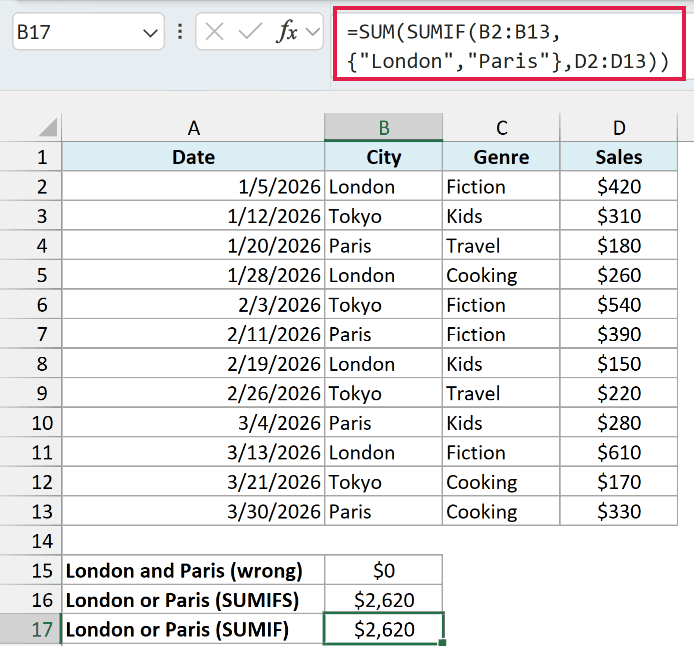
It also gives $2,620. The only difference is the argument order.
So yes, SUMIF can handle two criteria when they’re OR conditions on the same column.
The SUMIFS version has one advantage: you can still add AND conditions on other columns alongside the OR list.
Build a Two-Way Summary Table With One SUMIFS Formula
If you’re using Microsoft 365, SUMIFS can build an entire summary table with a single formula.
SUMIF can spill a one-column list this way, but not a two-way table, because it only has one condition.
Below is the same dataset. On the right, I have the cities in F2:F4 and the genres in G1:J1, and I want the total sales for every city and genre combination.
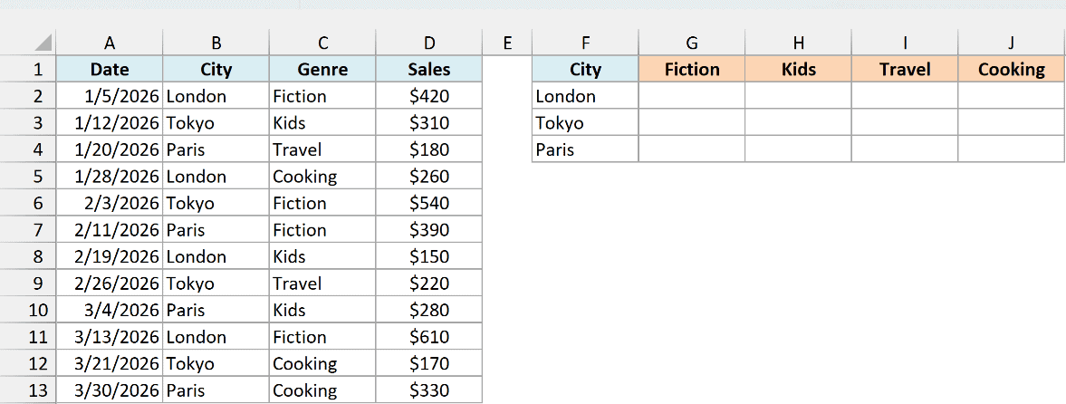
Here is the formula I entered in cell G2:
=SUMIFS(D2:D13,B2:B13,F2:F4,C2:C13,G1:J1)
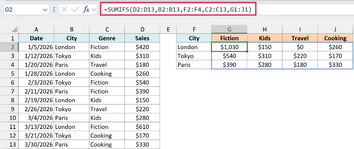
The formula spills across the whole table automatically, from G2 to J4.
The city criteria (F2:F4) run down the rows, and the genre criteria (G1:J1) run across the columns.
Excel pairs them up and calculates a separate total for each of the 12 combinations.
The $0 for London Travel is correct, since there are no Travel sales in London in this data.
Pro Tip: In Excel 2019 or earlier, use =SUMIFS($D$2:$D$13,$B$2:$B$13,$F2,$C$2:$C$13,G$1) in G2 and copy it across and down the table.
What Neither SUMIF Nor SUMIFS Can Do
SUMIF and SUMIFS follow the same criteria rules, so they also share the same limitations.
The main one is that the criteria range has to be an actual range of cells. You can’t run a function on it first, like MONTH() to get the month from each date.
Below is the same dataset. I want the total sales for March.
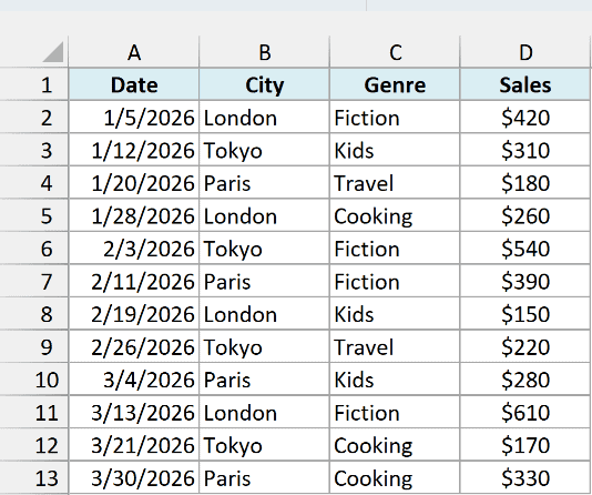
A formula like =SUMIF(MONTH(A2:A13),3,D2:D13) won’t work. Excel shows an error message and won’t let you enter it.
Here is a formula that works, using SUMPRODUCT instead:
=SUMPRODUCT((MONTH(A2:A13)=3)*D2:D13)
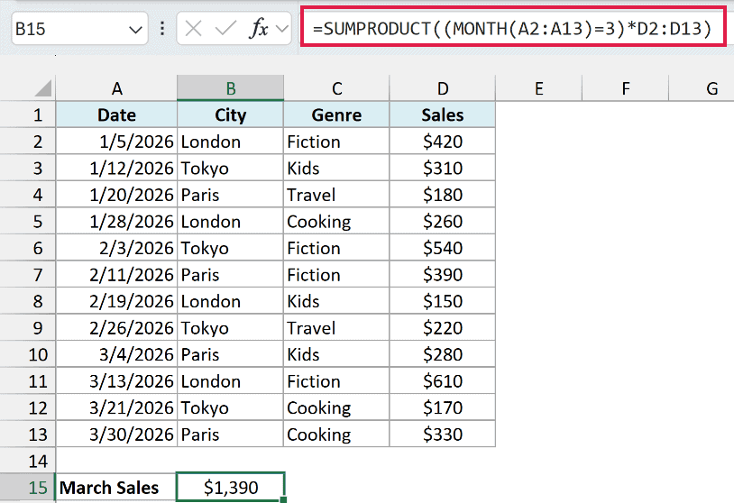
This gives $1,390.
MONTH(A2:A13)=3 returns TRUE for the March dates and FALSE for the rest. Multiplying by D2:D13 turns those into the sales amount or 0, and SUMPRODUCT adds them up.
For a simple month like this, you could also use SUMIFS with a start and end date, like in the date example above.
SUMPRODUCT becomes the better option when the condition needs a calculation that no date range can express.
Important: SUMIF and SUMIFS both return #VALUE! when they refer to another workbook that is closed. Open that workbook, or use SUMPRODUCT, which works with closed files.
In this article, I showed you the differences between SUMIF and SUMIFS.
These include the flipped argument order, mismatched range sizes, OR logic, and one-formula summary tables.
I hope you found this article helpful.
Other Excel Articles You May Also Like:
- COUNTIFS Function in Excel
- AVERAGEIFS Function in Excel
- SUM Based on Partial Text Match in Excel (SUMIF)
- Count Between Two Numbers in Excel (COUNTIF / COUNTIFS)
- How to Sum Only Positive or Negative Numbers in Excel (Easy Formula)
- How to Use Multiple Criteria in Excel COUNTIF and COUNTIFS Function
- 20 Advanced Excel Functions and Formulas (for Excel Pros)
- How to Sum a Column in Excel (5 Really Easy Ways)
