IFNA Function in Excel

The IFNA function in Excel lets you replace the #N/A error with a value or message of your choice.

Lookup functions like VLOOKUP and XMATCH return #N/A when they can’t find a match, so that’s where you’ll use IFNA most.

Unlike IFERROR, it only catches #N/A and lets every other error through, so a real mistake in your data still shows up.

In this article, I’ll show you how to use IFNA with six examples, from a simple VLOOKUP fix to looking up a value in two lists.

IFNA Function Syntax

Here is the syntax of the IFNA function:

=IFNA(value,value_if_na)

• value – the formula or value you want to check for the #N/A error. This is usually a lookup formula. If it isn’t #N/A, IFNA returns this result unchanged.
• value_if_na – what to return when value gives #N/A. It can be text in double quotes, a number, a cell reference, or another formula.

If you want the cell to look empty when there’s no match, use a pair of double quotes ("") as value_if_na.

Leaving value_if_na blank, as in =IFNA(VLOOKUP(...),), or pointing it at an empty cell shows 0 instead.

The IFNA function works in Excel 2013 and later, including Excel 365, 2024, 2021, 2019, 2016, Mac, and the web.

When to Use the IFNA Function

Use this function when you need to:

• Show a friendly message instead of #N/A when a lookup can’t find a value
• Return 0 for missing items so your calculations keep working
• Handle #N/A from functions that have no “not found” option, such as VLOOKUP, MATCH, and XMATCH
• Hide “not found” results while still seeing real errors like #VALUE!
• Check a second list when a value isn’t in the first one

Let me show you a few practical examples of how to use the IFNA function.

Example 1: IFNA with VLOOKUP to Replace #N/A with Text

Let’s start with the most common use.

VLOOKUP has no built-in way to deal with a value it can’t find, so it returns #N/A, and IFNA is how you clean that up.

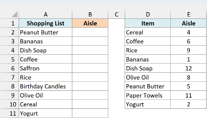
Below I have a shopping list and the store’s list of items with their aisle numbers, and I want to get the aisle for each item in column B.

Here is the formula:

=IFNA(VLOOKUP(A2:A11,D2:E10,2,FALSE),"Ask staff")

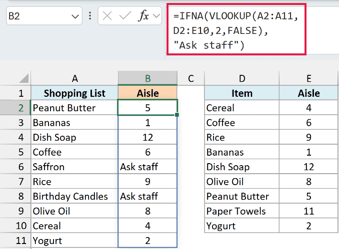
In the above formula, VLOOKUP looks for each item from A2:A11 in the store list (D2:E10) and returns the aisle number from its second column.

Saffron and Birthday Candles aren’t in the store list, so VLOOKUP returns #N/A for them. IFNA catches those two errors and shows “Ask staff” instead.

Since A2:A11 is a whole range, this one formula in B2 returns all ten results, and they spill down to B11. If any cell in B3:B11 already has something in it, you get a #SPILL! error instead, so keep that range empty.

If you are using Excel 2019 or earlier, enter the below formula in cell B2 and then copy it down the range:

=IFNA(VLOOKUP(A2,$D$2:$E$10,2,FALSE),"Ask staff")

Pro Tip: If you have Excel 2021 or later (including 365), XLOOKUP can do this without IFNA. Its fourth argument, if_not_found, sets what to return when there’s no match, so =XLOOKUP(A2:A11,D2:D10,E2:E10,"Ask staff") gives the same result.

Example 2: Return 0 Instead of #N/A in a Calculation

Now let’s put IFNA inside a calculation.

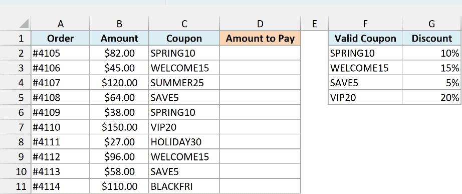
Below I have a list of online orders with the coupon code each customer typed in, plus a table of valid coupons and their discounts, and I want the amount to pay after the discount in column D.

Here is the formula:

=B2:B11*(1-IFNA(VLOOKUP(C2:C11,F2:G5,2,FALSE),0))

How this formula works:

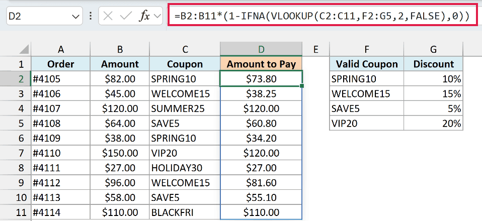
• VLOOKUP(C2:C11,F2:G5,2,FALSE) finds each coupon in the valid list and returns its discount. SUMMER25, HOLIDAY30, and BLACKFRI aren’t valid codes, so these three give #N/A.
• IFNA(...,0) turns each of those #N/A errors into 0, which means no discount.
• Subtracting the discount from 1 gives the share of the price the customer pays, and B2:B11* multiplies each order amount by that share. So the three orders with a bad code pay the full amount, like $120.00 for order #4107.

Important: If value_if_na is text, like “Invalid code”, Excel tries to multiply that text by the order amount, and those rows show #VALUE!. So when the IFNA result feeds a calculation, use a number such as 0.

If you are using Excel 2019 or earlier, enter the below formula in cell D2 and then copy it down the range:

=B2*(1-IFNA(VLOOKUP(C2,$F$2:$G$5,2,FALSE),0))

With XLOOKUP, the 0 goes straight into if_not_found: =B2:B11*(1-XLOOKUP(C2:C11,F2:F5,G2:G5,0)).

Example 3: IFNA with XMATCH to Find a Position

IFNA is just as handy with XMATCH, which tells you where something sits in a list.

Below I have everyone who signed up for a fun run, plus the names of the runners in the order they crossed the finish line, and I want each person’s finish position in column B.

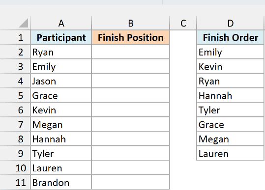
Here is the formula:

=IFNA(XMATCH(A2:A11,D2:D9),"DNF")

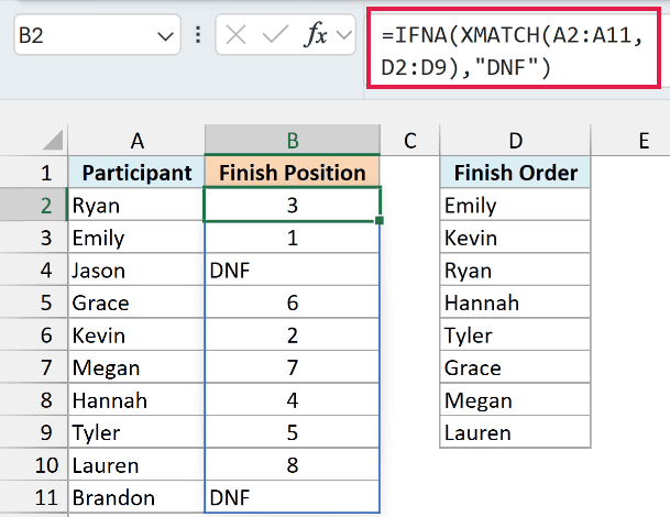
Here, XMATCH looks for each name from A2:A11 in the finish order list and returns its position. Ryan is third in that list, so he gets 3.

Jason and Brandon never crossed the finish line, so XMATCH can’t find them and returns #N/A. IFNA shows DNF (did not finish) for them instead.

XMATCH has no argument for a missing value, so there’s no way to get DNF out of XMATCH alone. Wrapping it in IFNA fills that gap.

The XMATCH function needs Excel 2021 or later (including 365). If you are using Excel 2019 or earlier, enter the below formula in cell B2 and then copy it down the range:

=IFNA(MATCH(A2,$D$2:$D$9,0),"DNF")

Example 4: IFNA vs IFERROR (Keep Real Errors Visible)

This next example shows the one big difference between IFNA and IFERROR.

Below I have a list of nightly hotel rates and a trip plan with the number of nights in each city, and I want the hotel cost for each city in column F.

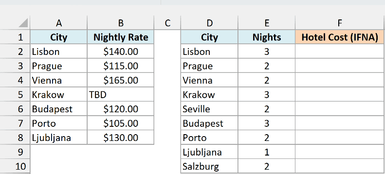
Here is the formula:

=IFNA(XLOOKUP(D2:D10,A2:A8,B2:B8)*E2:E10,"City not listed")

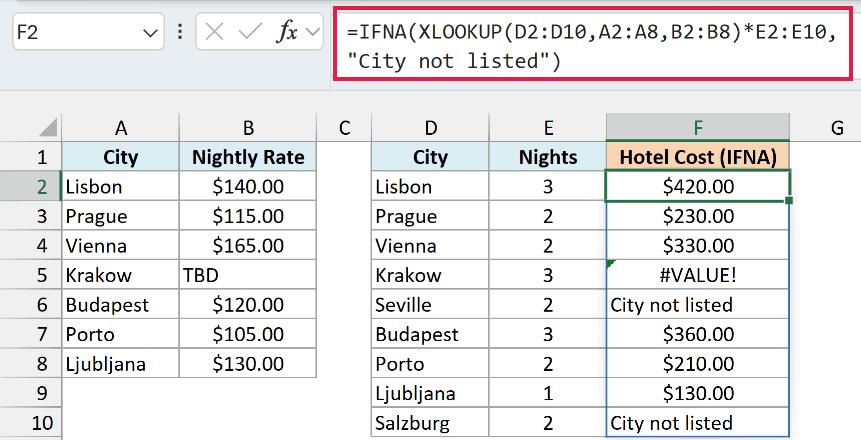
XLOOKUP looks up each city from D2:D10 in the city column of the rate list (A2:A8) and returns its nightly rate from B2:B8. That rate is then multiplied by the number of nights in E2:E10.

Seville and Salzburg aren’t in the rate list, so XLOOKUP returns #N/A for them, and IFNA shows “City not listed”.

Krakow is a different story. It’s in the rate list, but its rate is still TBD, so multiplying that text by 3 nights gives a #VALUE! error.

IFNA leaves that error alone, because it only handles #N/A. That’s what you want here, since the #VALUE! tells you a rate still needs filling in.

Now here is the same formula with IFERROR, in column G:

=IFERROR(XLOOKUP(D2:D10,A2:A8,B2:B8)*E2:E10,"City not listed")

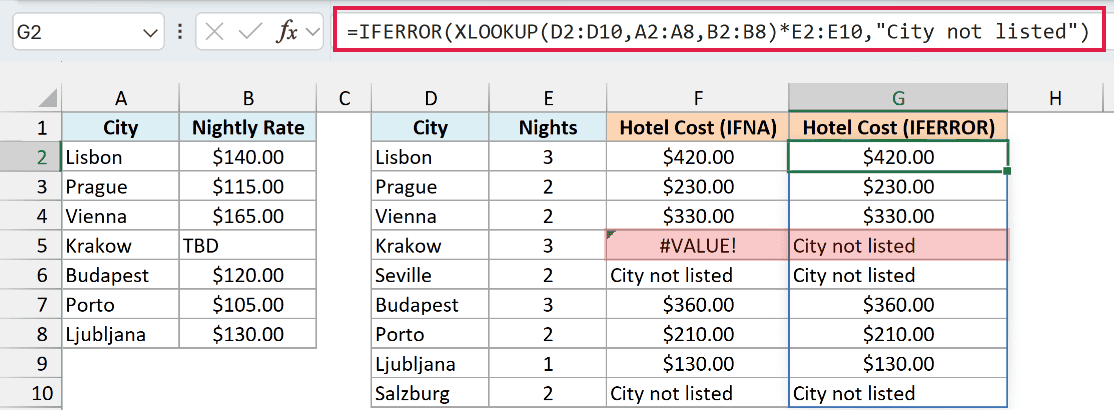
IFERROR catches every error, not just #N/A. So Krakow also shows “City not listed”, which is wrong, because Krakow is in the list and only its rate is missing.

Important: IFERROR can hide a real data problem. If you SUM column G, you get $1,680.00 with Krakow quietly left out, while a SUM of column F shows #VALUE! until you fix the rate.

You might wonder why IFNA wraps the whole calculation instead of using XLOOKUP’s own if_not_found argument. If XLOOKUP returned “City not listed”, that text would get multiplied by the nights too, and you’d get #VALUE! for the missing cities.

So for lookups, use IFNA when you only want to handle missing values, and keep IFERROR for the times you really do want to hide every error.

XLOOKUP needs Excel 2021 or later (including 365). If you are using Excel 2019 or earlier, enter the below IFNA formula in cell F2 and then copy it down the range:

=IFNA(VLOOKUP(D2,$A$2:$B$8,2,FALSE)*E2,"City not listed")

Example 5: IFNA with an Approximate Match VLOOKUP

Let’s step it up with an approximate match, where #N/A shows up for a different reason.

Below I have a list of loyalty program members with their points, plus a reward table that shows the minimum points for each tier, and I want each member’s reward in column C.

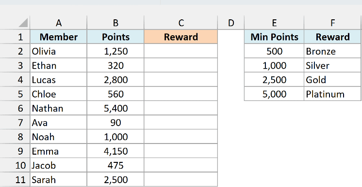
Here is the formula:

=IFNA(VLOOKUP(B2:B11,E2:F5,2,TRUE),"No reward yet")

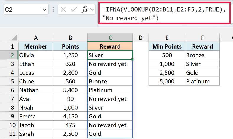
With TRUE as the last argument, VLOOKUP looks for the largest Min Points value that’s less than or equal to each member’s points. Olivia has 1,250 points, so she lands on the 1,000 tier and gets Silver.

Ethan (320), Ava (90), and Jacob (475) are all below the lowest tier of 500. There’s nothing in the table for VLOOKUP to land on, so it returns #N/A, and IFNA shows “No reward yet”.

For an approximate match like this, the Min Points column has to be sorted from smallest to largest. If it isn’t, VLOOKUP can return the wrong reward.

If you are using Excel 2019 or earlier, enter the below formula in cell C2 and then copy it down the range:

=IFNA(VLOOKUP(B2,$E$2:$F$5,2,TRUE),"No reward yet")

With XLOOKUP, =XLOOKUP(B2:B11,E2:E5,F2:F5,"No reward yet",-1) gives the same result without IFNA. The -1 match mode tells XLOOKUP to use the next smaller value when there’s no exact match.

Example 6: Use IFNA to Look Up in Two Lists

Finally, let’s use IFNA to check a second list when a name isn’t in the first one.

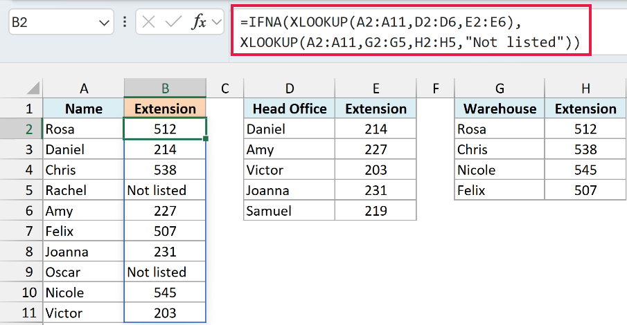
Below I have a list of names, plus two phone lists (one for the head office and one for the warehouse), and I want each person’s extension in column B, from whichever list they’re on.

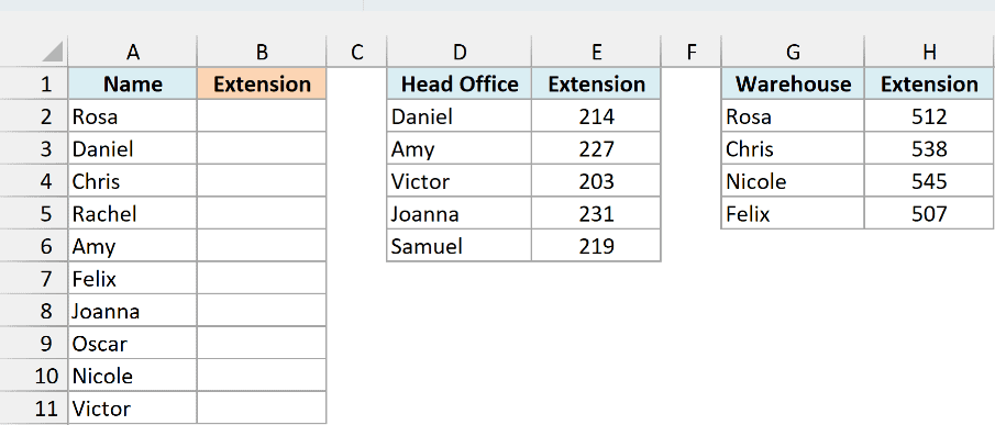
Here is the formula:

=IFNA(XLOOKUP(A2:A11,D2:D6,E2:E6),XLOOKUP(A2:A11,G2:G5,H2:H5,"Not listed"))

How this formula works:

• XLOOKUP(A2:A11,D2:D6,E2:E6) looks for each name in the Head Office list. Daniel, Amy, Joanna, and Victor are found there, and everyone else gets #N/A.
• IFNA sends only those #N/A results to the second XLOOKUP, which checks the Warehouse list. That’s how Rosa gets 512 and Nicole gets 545.
• Rachel and Oscar aren’t in either list, so the second XLOOKUP’s if_not_found argument returns “Not listed”.

Important: Putting the second XLOOKUP inside the first one’s if_not_found argument looks simpler, but with a range like A2:A11 it gives wrong answers. Every name missing from Head Office gets 512, the first result of the second lookup.

If you are using Excel 2019 or earlier, enter the below formula in cell B2 and then copy it down the range:

=IFNA(VLOOKUP(A2,$D$2:$E$6,2,FALSE),IFNA(VLOOKUP(A2,$G$2:$H$5,2,FALSE),"Not listed"))

So these are six ways you can use the IFNA function in Excel to handle lookups that come up empty.

The main thing to remember is that IFNA only touches #N/A, so any other error is still there to warn you. I hope you found this article helpful.

List of All Excel Functions

Other Excel Articles You May Also Like:

• Use IFERROR with VLOOKUP to Get Rid of #N/A Errors
• VLOOKUP Not Working? (10 Common Fixes)
• IS Functions in Excel (8 Examples)
• 20 Advanced Excel Functions and Formulas (for Excel Pros)
• Lookup the Second, the Third, or the Nth Value in Excel
• How to Compare Two Columns in Excel (for matches & differences)