VDB Function in Excel

The VDB function in Excel calculates the depreciation of an asset using the declining balance method, for any stretch of time you pick. That can be one year, a few years together, a single month, or even part of a year.

VDB stands for variable declining balance. By default, it uses the double declining rate and switches to straight-line depreciation once that gives a bigger number, so the asset ends up exactly at its salvage value.

In this article, I’ll show you how the VDB function works, starting with a simple first-year number and building up to full schedules, mid-year purchases, and the optional arguments.

VDB Function Syntax

Here is the syntax of the VDB function:

=VDB(cost, salvage, life, start_period, end_period, [factor], [no_switch])

• cost – the price you paid for the asset.
• salvage – the value of the asset at the end of its life. It can be 0.
• life – the number of periods over which the asset is depreciated (its useful life).
• start_period – the point in the asset’s life where the calculation starts.
• end_period – the point in the asset’s life where the calculation stops.
• factor – (optional) the rate at which the balance declines. If you leave it out, Excel uses 2, which is the double declining balance method.
• no_switch – (optional) set it to TRUE to stop VDB from switching to straight-line depreciation. FALSE, or leaving it out, lets it switch.

The start_period and end_period are points in time, not period numbers. 0 is the day you bought the asset and 1 is the end of the first period, so the depreciation for year 3 is the stretch from 2 to 3.

The VDB function works in all Excel versions, including 365, 2024, 2021, 2019, 2016, Mac, and the web. The examples that build a whole schedule with one spilling formula need Excel 365 or Excel 2021 and later.

When to Use the VDB Function

Use this function when you need to:

• Get the depreciation for a single year or month using the declining balance method
• Build a depreciation schedule that ends exactly at the salvage value
• Get the total depreciation for a range of periods, such as years 2 to 4, in one formula
• Depreciate an asset that was bought partway through the year
• Use a declining rate other than double, such as 150%

Let me show you a few practical examples of how to use the VDB function.

Example 1: Calculate First-Year Depreciation With VDB

Let’s start with a simple example.

Below are the details of a commercial dishwasher a restaurant bought, and I want to get its depreciation for the first year in cell B6.

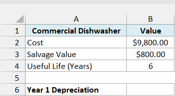
Here is the formula:

=VDB(B2,B3,B4,0,1)

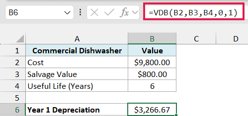
This gives us $3,266.67.

The start_period is 0 (the day the dishwasher was bought) and the end_period is 1 (the end of the first year). So VDB returns the depreciation for the whole first year.

Since I didn’t give a factor, VDB uses the double declining rate, which is 2 divided by the life, applied to whatever value is left each year. In the first year, that’s 2/6 of the full $9,800 cost, which is $3,266.67.

Important: If you use 1 as both the start_period and the end_period for the first year, VDB returns 0, because the start and end are the same point. The first year always starts at 0.

Example 2: Create a Depreciation Schedule With One Formula

Now let’s get the depreciation for every year of an asset’s life.

Below are the details of a farm tractor, with the years 1 to 8 in column A, and I want the depreciation for each year in column B.

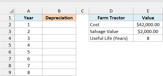
Here is the formula:

=VDB(E2,E3,E4,A2:A9-1,A2:A9)

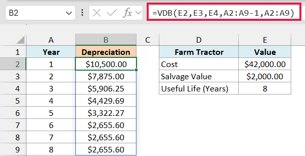
This one formula spills the depreciation for all eight years down column B.

How this formula works:

• A2:A9-1 gives the start of each year (0, 1, 2, and so on up to 7).
• A2:A9 gives the end of each year (1, 2, 3, and so on up to 8).
• VDB calculates one value for each pair, so year 1 runs from 0 to 1, year 2 from 1 to 2, and so on.

Now look at years 6, 7, and 8. They’re all $2,655.60, because VDB switched to straight-line depreciation once spreading the remaining value evenly gave more than the declining balance.

Thanks to that switch, the eight years add up to $40,000, which is exactly the $42,000 cost minus the $2,000 salvage value.

The DDB function never switches, so with the same numbers it stops at $37,795.26 and leaves the tractor above its salvage value.

If you’re using Excel 2019 or earlier, enter the below formula in cell B2 and then copy it down to B9:

=VDB($E$2,$E$3,$E$4,A2-1,A2)

The other schedules in this article work the same way in older versions. Lock the input cells with dollar signs and point to that row’s own period cells.

Example 3: Get the Depreciation for Years 2 to 4

VDB can also give you the total depreciation across several periods in one formula. The DB and DDB functions can’t do this, since they return one period at a time.

Below are the details of a food truck, with a start period of 1 and an end period of 4, and I want the total depreciation for years 2 to 4 in cell B8.

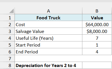
Here is the formula:

=VDB(B2,B3,B4,B5,B6)

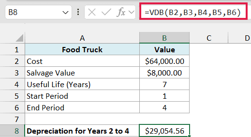
This gives us $29,054.56.

A start_period of 1 is the end of year 1, and an end_period of 4 is the end of year 4. So the stretch between them covers years 2, 3, and 4.

You’d get the same $29,054.56 if you worked out the depreciation for years 2, 3, and 4 separately and added them up. VDB just does it in one go.

Pro Tip: To get the book value (what the asset is still worth on the books) after a few years, subtract the depreciation from 0 to that year from the cost. For example, =B2-VDB(B2,B3,B4,0,4) returns $16,659.73, the food truck’s value at the end of year 4.

Example 4: Calculate Monthly Depreciation

Here’s another practical scenario, where you need the depreciation month by month.

Below are the details of a 3D printer with a useful life of 5 years, with the months 1 to 12 in column A, and I want the depreciation for each of the first 12 months in column B.

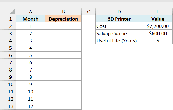
Here is the formula:

=VDB(E2,E3,E4*12,A2:A13-1,A2:A13)

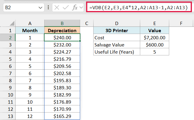
The periods here are months, so the life has to be in months too. E4*12 turns the 5-year life into 60 months, and A2:A13-1 and A2:A13 give the start and end of each month.

These 12 months add up to $2,406.49. That’s less than the $2,880 you get for the whole first year with yearly periods, because a monthly schedule reduces the value every month instead of once a year.

So use the period that matches how you report depreciation.

Important: If you leave the life in years while the periods are months, VDB treats each month as a full year. Month 1 would then show $2,880 (the whole first year’s depreciation) instead of $240.

Example 5: Depreciation for an Asset Bought Mid-Year

Let’s step it up with an asset that was bought partway through the year.

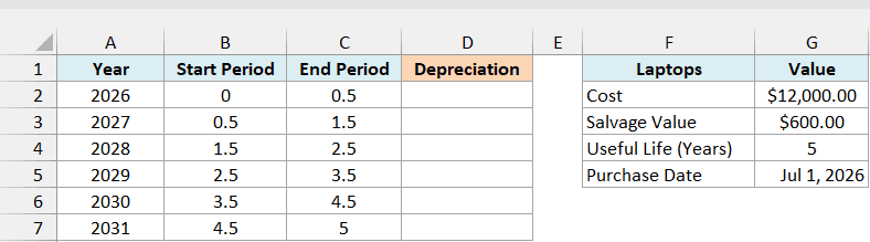
Below are the details of laptops a design studio bought on July 1, 2026, with the start and end period for each calendar year in columns B and C, and I want the depreciation for each year in column D.

Here is the formula:

=VDB(G2,G3,G4,B2:B7,C2:C7)

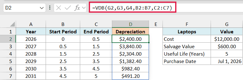
Since the laptops were bought in the middle of 2026, they’re only used for half a year in 2026. So 2026 runs from 0 to 0.5, 2027 runs from 0.5 to 1.5, and so on.

The 5-year life ends halfway through 2031, which is why the last year runs from 4.5 to 5. VDB accepts these fractional periods and works out the depreciation for each stretch.

For 2026, you get $2,400, which is half of the $4,800 a full first year would give. The six years add up to $11,400, the $12,000 cost minus the $600 salvage value.

If an asset is bought on April 1 instead, it’s used for 9 months in the first year. So the first year runs from 0 to 0.75 (9 divided by 12), and every later year shifts by the same amount.

Example 6: Use a Different Factor (150% Declining Balance)

By default, VDB uses double declining balance. You can change that rate with the factor argument.

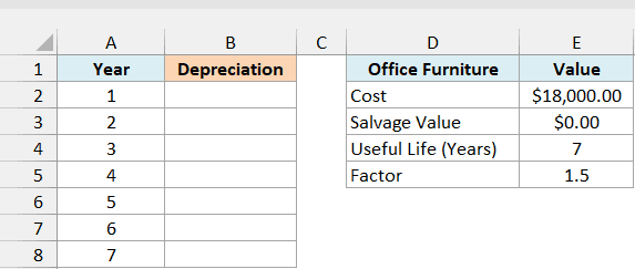
Below are the details of office furniture with a factor of 1.5 in cell E5, and I want a 150% declining balance schedule for its 7-year life in column B.

Here is the formula:

=VDB(E2,E3,E4,A2:A8-1,A2:A8,E5)

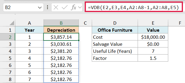
With a factor of 1.5, the furniture loses 1.5/7 of its remaining value each year instead of 2/7. So year 1 gives $3,857.14, compared to $5,142.86 with the default factor of 2.

From year 4, the values flatten out at $2,182.76 because VDB switches to straight-line. A lower factor keeps the early-year depreciation smaller, which leaves more value to spread over the later years.

Since the factor sits in its own cell, you can change it to 1.25 or 2 and the whole schedule updates.

Example 7: Stop VDB From Switching to Straight Line

In the tractor and office furniture schedules, VDB switched to straight-line depreciation near the end. Let me show you what happens when you turn that off.

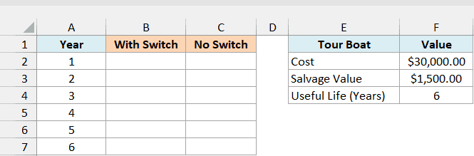
Below are the details of a tour boat, with the years 1 to 6 in column A, and I want the depreciation for each year with the default switch in column B and without it in column C.

Here is the formula:

=VDB(F2,F3,F4,A2:A7-1,A2:A7)

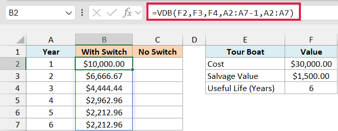
In years 5 and 6, VDB switches to straight-line and gives $2,212.96 for each year. The six years add up to $28,500, which is the cost minus the salvage value.

Now let’s set no_switch to TRUE and get the schedule without the switch in column C. Here is the formula:

=VDB(F2,F3,F4,A2:A7-1,A2:A7,2,TRUE)

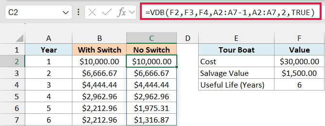
Column C keeps using the declining balance method, so years 5 and 6 drop to $1,975.31 and $1,316.87. These six years add up to only $27,366.26, so the boat is still on the books at $2,633.74, above its $1,500 salvage value.

These match what the DDB function returns for the same boat.

Important: Since no_switch comes after factor, you need to enter the factor too (I used 2, the default). If you skip it with two commas, like A2:A7,,TRUE, VDB returns 0 for every year.

So these are some examples of how to use the VDB function in Excel. I showed you how to get the depreciation for a single year, a range of years, months, and partial years, and how the factor and no_switch arguments change the schedule.

I hope you found this Excel tutorial useful.

List of All Excel Functions

Other Excel Articles You May Also Like:

• DB Function in Excel
• AMORDEGRC guide
• How to use AMORLINC in Excel
• How to use SYD in Excel