

The ACCRINTM function in Excel calculates the interest on an investment that pays all its interest at maturity. It uses the issue date, maturity date, annual rate, and face value to work out the amount.
It returns the interest amount only. In this tutorial, I’ll show you how to calculate it for one investment or a list, compare day-count methods, and add the principal to get the final payment.
Follow along with the example file
ACCRINTM Function Examples.xlsx
ACCRINTM Function Syntax
Here is the syntax of the ACCRINTM function:
=ACCRINTM(issue, settlement, rate, par, [basis])
- issue is the date the investment starts earning interest. Supply a real Excel date, usually a cell reference.
- settlement is the maturity date for this function, despite the argument’s name. This is the date the interest is paid.
- rate is the annual interest rate. Enter a percentage such as 4.8% or its decimal equivalent, 0.048.
- par is the face value, or principal amount, on which interest is calculated. For example, use 12500 for an investment with a face value of $12,500.
- basis is an optional number from 0 to 4 that controls how Excel counts days for the interest calculation.
If you leave out basis, Excel uses 0, which means US (NASD) 30/360. The choices below can produce different interest amounts for the same dates, so use the method specified in the investment’s terms.
| Basis | Day-count method |
|---|---|
| 0 or omitted | US (NASD) 30/360: adjusted 30-day months and a 360-day year |
| 1 | Actual/actual: actual days, with the year length reflecting leap years |
| 2 | Actual/360: actual days divided by 360 |
| 3 | Actual/365: actual days divided by 365 |
| 4 | European 30/360: 30-day months and a 360-day year, with different month-end rules from basis 0 |
Excel uses a par value of 1,000 if you leave the fourth argument’s slot empty. Entering your actual principal explicitly makes the calculation easier to check and avoids accidentally using that default.
The ACCRINTM function works in Excel 365, 2024, 2021, 2019, and 2016, including supported Mac versions. The spilling examples below need dynamic-array Excel, such as 365, 2024, or 2021.
When to Use the ACCRINTM Function
Use this function when you need to:
- Calculate interest on an investment that pays its interest once, at maturity.
- Work out the interest for several such investments in a maturity schedule.
- Check how the day-count basis affects an interest calculation.
- Calculate a maturity payment that includes both principal and interest.
Let’s start with one investment, then work through the other examples. The example file has a separate sheet for each one.
Example 1: Calculate Interest at Maturity
Below is a $12,500 investment earning 4.8% annually from 10-Feb-2026 to 10-Aug-2026, and I want to calculate its interest in cell B8.
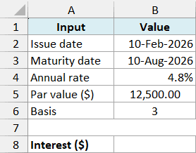
Enter this formula in cell B8:
=ACCRINTM(B2,B3,B4,B5,B6)
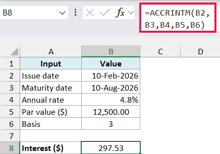
The formula returns $297.53 when the cell is formatted to show two decimal places. It uses the dates in B2 and B3, the annual rate in B4, the principal in B5, and the basis in B6.
Here, basis 3 means Actual/365. There are 181 days between the two dates, so the calculation is $12,500 × 4.8% × 181 ÷ 365, giving $297.5342 before display rounding.
Important: Enter the rate as 4.8% or 0.048, not 4.8. Excel treats 4.8 as 480%, which makes the interest 100 times too large.
The dates must be real Excel dates. If a date is unrecognized text, the formula can return #VALUE!; the DATE function can create a date from separate year, month, and day values.
A maturity date before the issue date produces #NUM!. You also get #NUM! when the rate or par value is zero or negative, or when the basis is outside 0 to 4.
Example 2: Calculate Interest for Several Investments
Now let’s calculate a whole list in one go. Below is a schedule of six investments that pay interest at maturity, and I want the interest for each investment in column E.
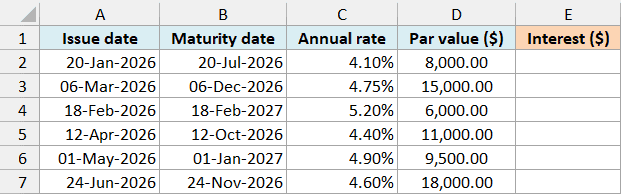
In Excel 365, 2024, or 2021, enter this formula in cell E2:
=ACCRINTM(A2:A7+0,B2:B7+0,C2:C7+0,D2:D7+0,3)
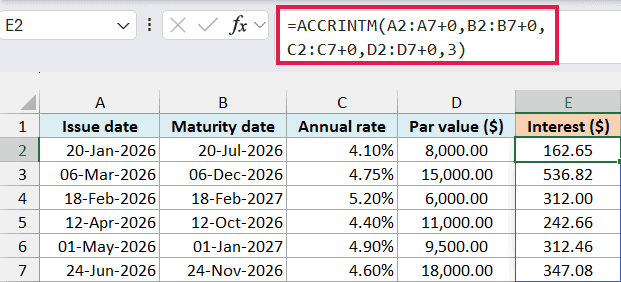
The formula spills six interest amounts into E2:E7. Each result uses the issue date, maturity date, rate, and par value from the same row, while the final argument applies Actual/365 to all six investments.
For the first investment, the result is $162.65. That comes from $8,000 × 4.1% × 181 ÷ 365, with the displayed amount rounded to two decimal places.
The +0 after each range matters here. ACCRINTM can return #VALUE! when given those ranges directly; adding zero converts each range to an array of numbers without changing its values, so the function can calculate one result per row.
Excel stores real dates as numbers, which is why the same conversion works for the two date columns. It doesn’t reliably fix dates stored as text, so make sure the dates are valid before using this formula.
If you get #SPILL!, clear anything blocking E3:E7 so the other results have room. If you add more investments below row 7, extend all four input ranges to include the new rows.
In Excel 2019 or earlier, enter this one-row formula in E2 and copy it down to E7:
=ACCRINTM(A2,B2,C2,D2,3)
The references change as you copy the formula, so each row uses its own investment details.
Example 3: Compare Day-Count Bases
The same rate and dates can give different results depending on the day-count basis.
Below is a $20,000 investment earning 5.4% from 29-Feb-2028 to 31-Aug-2028, and I want to compare its interest under all five bases in column C.
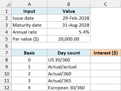
In Excel 365, 2024, or 2021, enter this formula in cell C8:
=ACCRINTM(B2,B3,B4,B5,A8:A12+0)
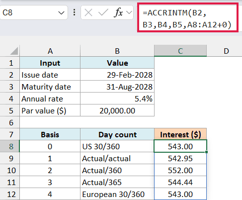
The formula keeps the investment details in B2:B5 the same and uses the five basis numbers in A8:A12. As in the previous example, +0 converts the range into a numeric array, so the five results spill into C8:C12.
There are 184 actual days between these dates. Because 2028 is a leap year, basis 1 uses 366 days for this period and returns $542.95, while basis 3 uses 365 and returns $544.44.
Basis 2 uses those same 184 days with a 360-day year, giving $552.00. The two 30/360 methods both return $543.00 for these dates, although their different month-end rules can give different answers for other date pairs.
Important: The largest result isn’t automatically the correct one. Use the basis specified in the investment’s terms; changing it just to increase the interest gives the wrong calculation for that investment.
In Excel 2019 or earlier, enter this formula in C8 and copy it down to C12:
=ACCRINTM($B$2,$B$3,$B$4,$B$5,A8)
The dollar signs keep the four investment inputs fixed as you copy down. The basis reference changes from A8 to A9, A10, and so on, giving one result for each method.
Example 4: Include Principal in the Maturity Payment
So far, the results show interest alone. Below is a $24,000 investment earning 5% from 15-Sep-2026 to 15-Mar-2027, and I want the total principal-plus-interest payment in cell B8.
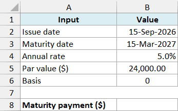
Enter this formula in cell B8:
=B5+ACCRINTM(B2,B3,B4,B5,B6)
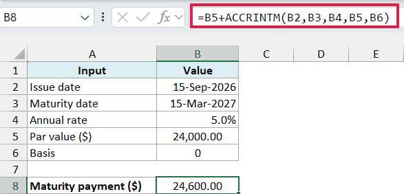
The formula returns $24,600.00. ACCRINTM calculates $600 in interest using basis 0, and the B5+ at the beginning adds the $24,000 principal exactly once.
This assumes the investment repays its full face value at maturity and has no fees or taxes deducted. Those amounts would need to be included separately if they apply to your payment.
ACCRINTM calculates simple interest, so it doesn’t add interest back to the principal during the investment. For a balance that earns interest on earlier interest, use a compound interest calculation instead.
In this tutorial, I showed you how to calculate interest at maturity, apply it to several investments, compare bases, and include principal in the final payment. For investments that pay interest periodically, the ACCRINT function handles that different payment pattern.
I hope you found this Excel tutorial useful.
Other Excel Articles You May Also Like:
