

The GCD function in Excel gives you the greatest common divisor of two or more numbers. That’s the biggest whole number that divides every one of them with nothing left over.
It’s handy whenever you want to split things into equal groups, find the largest size that fits evenly, or reduce a ratio like 600:400 down to 3:2.
If you give GCD two columns, it returns one GCD for all the numbers in both columns together, not one result per row. I’ll show you how to handle that, along with a few other traps that give a wrong answer without any error.
Follow along with the example file
GCD Function Examples.xlsx
GCD Function Syntax
Here is the syntax of the GCD function:
=GCD(number1, [number2], ...)
- number1 is the first number, cell, or range you want the greatest common divisor of.
- [number2], … are optional extra numbers, cells, or ranges. You can give GCD up to 255 arguments in total.
GCD works with whole numbers. If you give it a decimal, it cuts off the decimal part instead of rounding, so =GCD(8.5,12.75) returns 4, the same as =GCD(8,12).
A negative number returns a #NUM! error, and text that isn’t a number returns a #VALUE! error.
A 0 doesn’t change the result, because every number divides 0. So =GCD(5,0) returns 5.
The GCD function works in Excel 365, 2024, 2021, 2019, 2016, and Excel for Mac.
When to Use the GCD Function
Use this function when you need to:
- Split several items into as many identical bags, boxes, or kits as possible, with nothing left over.
- Find the largest size that fits two measurements exactly, like a square tile for a floor.
- Reduce a ratio or a fraction to its simplest form.
- Pick one pack size that works for every order in a list.
Let me show you a few practical examples of how to use the GCD function.
Example 1: Find the GCD of a List of Numbers
Let’s start with a simple example.
Below is a list of party favors with how many of each item I have, and I want the largest number of identical favor bags I can make in cell F1 and how many of each item goes in each bag in column C.
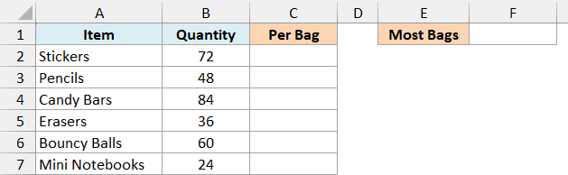
Here is the formula to enter in cell F1:
=GCD(B2:B7)
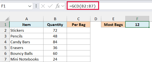
GCD looks at all six quantities in B2:B7 and returns 12. That’s the largest number that divides 72, 48, 84, 36, 60, and 24 with nothing left over, so I can make 12 identical bags.
Important: If any cell in the range has text in it, even a dash or “N/A”, GCD returns a #VALUE! error for the whole range. A blank cell is fine, since GCD ignores it.
Now, to see how many of each item goes into a bag, here is the formula to enter in cell C2:
=B2:B7/F1
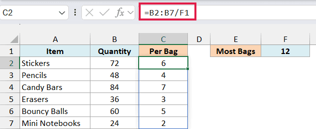
This divides every quantity by the 12 bags in F1, and the results spill down to C7. So each bag gets 6 stickers, 4 pencils, 7 candy bars, and so on.
If you are using Excel 2019 or earlier, enter the below formula in cell C2 and then copy it down to C7:
=B2/$F$1
Example 2: Find the Largest Square Tile for a Room
Here’s another practical scenario.
Below is a list of rooms with their length and width in inches, and I want the largest square tile that covers each floor exactly, with no cut tiles, in column D.
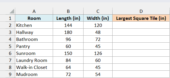
Here is the formula to enter in cell D2, which you then copy down to D9:
=GCD(B2,C2)
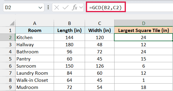
For the kitchen, GCD finds the largest number that divides both 144 and 120, which is 24. So 24-inch tiles fit the kitchen exactly, 6 tiles one way and 5 the other.
The walk-in closet returns 1, because 64 and 45 have no common divisor other than 1. The only square tile that fits that floor exactly is a 1-inch one.
Here we keep this as a per-row formula because GCD always returns one number for everything you give it.
Important: Don’t use =GCD(B2:B9,C2:C9) to get all the rooms at once. It returns a single 1, the GCD of all 16 numbers together, instead of one result for each room.
If you want one formula that spills a result for every row, you can wrap GCD in the BYROW function, which I cover in Example 6.
Example 3: Simplify Ratios With the GCD Function
Now let’s use GCD to clean up some ratios.
Below is a list of drinks with how much juice and sparkling water goes into each, and I want the juice-to-water ratio in its simplest form in column D.
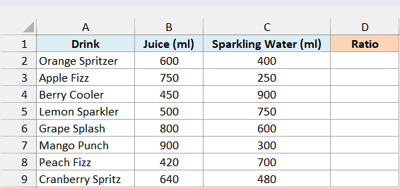
Here is the formula to enter in cell D2, which you then copy down to D9:
=LET(g,GCD(B2,C2),B2/g&":"&C2/g)
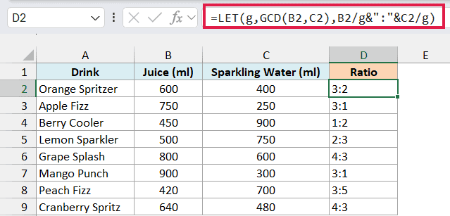
How this formula works:
- GCD(B2,C2) finds the largest number that divides both amounts. For the Orange Spritzer, 600 and 400 have a GCD of 200.
- LET stores that result as g, so the formula only works it out once.
- B2/g&”:”&C2/g divides both amounts by 200 and joins them with a colon, which gives 3:2.
The result is text, so you can’t do math with it. If you need the parts as numbers, divide each amount by the GCD in its own column.
If one of the two cells is empty, GCD ignores it and works with the other amount alone, so you get a ratio like 1:0. If both are empty, GCD has no numbers to work with and returns a #VALUE! error.
So fill in both amounts on every row before you copy the formula down.
The LET function needs Excel 365 or 2021 and later. If you are using Excel 2019 or earlier, enter the below formula in cell D2 and then copy it down to D9:
=B2/GCD(B2,C2)&":"&C2/GCD(B2,C2)
Example 4: Use GCD With FILTER for a Chosen Product
Let’s step it up with a formula that only looks at some of the rows.
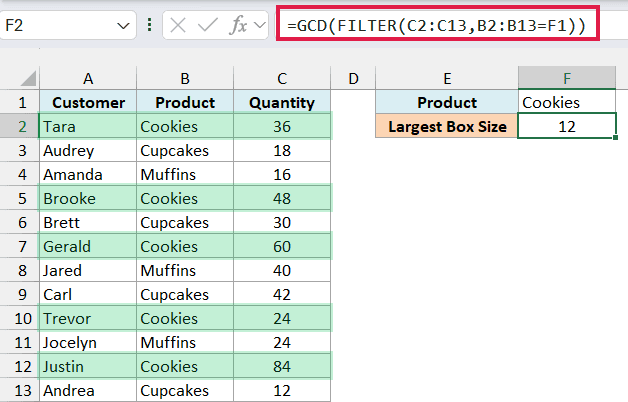
Below is a list of bakery orders with the customer, the product, and the quantity, and I want the largest box size that packs every order of the product in cell F1 with no leftovers, in cell F2.
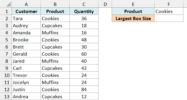
Here is the formula to enter in cell F2:
=GCD(FILTER(C2:C13,B2:B13=F1))
How this formula works:
- FILTER(C2:C13,B2:B13=F1) pulls out only the quantities where the product is Cookies, which are 36, 48, 60, 24, and 84.
- GCD then finds the largest number that divides all five, which is 12. So boxes of 12 cookies pack every cookie order exactly.
Change F1 to Cupcakes and the result changes to 6, and for Muffins it’s 8.
If no order matches the product in F1, FILTER has nothing to return and you get a #CALC! error.
The FILTER function needs Excel 365 or 2021 and later. If you are using Excel 2019 or earlier, enter the below formula in cell F2 and press Control + Shift + Enter:
=GCD(IF(B2:B13=F1,C2:C13,0))
The 0 at the end matters. IF puts a 0 in place of every order that isn’t Cookies, and GCD ignores zeros, but without it IF returns FALSE for those rows and GCD gives a #VALUE! error.
Example 5: Find the GCD of Decimal Numbers
Here’s a scenario where GCD gives you a wrong answer without any error.
Below is a list of ribbon rolls with their length in feet, some of them in half feet, and I want the longest piece I can cut every ribbon into with nothing left over, in column E.
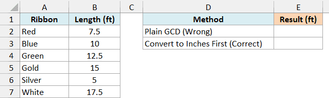
First, here is what happens with a plain GCD formula in cell E2:
=GCD(B2:B7)
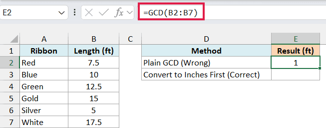
This returns 1, which is wrong. GCD cuts 7.5 down to 7, 12.5 down to 12, and 17.5 down to 17, and then finds the GCD of those whole numbers instead.
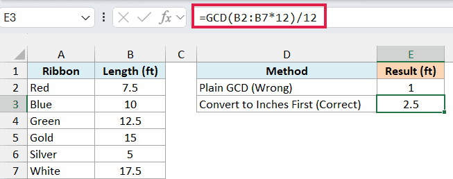
The fix is to turn the lengths into whole numbers first. Here is the formula to enter in cell E3:
=GCD(B2:B7*12)/12
How this formula works:
- B2:B7*12 turns every length into inches, so 7.5 feet becomes 90 inches. Now every value is a whole number.
- GCD finds the largest number that divides all six inch values, which is 30.
- /12 turns the 30 inches back into feet, which gives 2.5. So every ribbon can be cut into 2.5-foot pieces with nothing wasted.
If you are using Excel 2019 or earlier, enter the below formula in cell E3 and press Control + Shift + Enter, since it does math on a whole range:
=GCD(B2:B7*12)/12
The trick works with any number that turns every value into a whole number, as long as you divide the result by the same number. Here 12 works because every length is a whole number of inches.
For values like 2.1 or 0.3 that aren’t whole inches, multiply by 10, 100, or 1000 instead, and divide by the same number at the end.
Important: Excel stores some decimals with a tiny error, so 0.29*100 can come out just under 29, and GCD then cuts it to 28 and gives a wrong answer. To avoid this, wrap the multiplication in ROUND, like =GCD(ROUND(B2:B7*100,0))/100.
Example 6: Simplify Ratios With Three or More Parts
In Example 3, we simplified a two-part ratio with a formula copied down the column. Now let’s do it for ratios with three parts, all with one formula.
Below is a list of trail mix recipes with the grams of nuts, raisins, and chocolate in each, and I want the simplest nuts-to-raisins-to-chocolate ratio for each mix in column E.
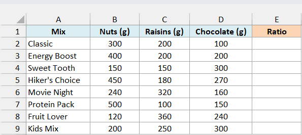
Here is the formula to enter in cell E2:
=BYROW(B2:D9,LAMBDA(r,TEXTJOIN(":",,r/GCD(r))))
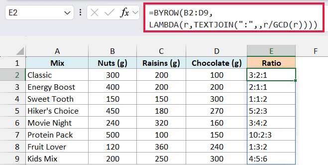
How this formula works:
- BYROW(B2:D9,…) goes through the table one row at a time and hands each row to the LAMBDA function.
- LAMBDA(r,…) names the current row r and runs the calculation after it on that row.
- GCD(r) finds the GCD of the three amounts in that row. For the Classic mix, 300, 200, and 100 have a GCD of 100.
- r/GCD(r) divides all three amounts by it, which gives 3, 2, and 1.
- TEXTJOIN(“:”,,…) joins those numbers with colons, so you get 3:2:1. The empty middle argument is TEXTJOIN‘s optional ignore-empty setting, left out here. BYROW then spills one ratio for every mix down to E9.
This formula doesn’t care how many columns you have. If you add a fourth ingredient in column E, change B2:D9 to B2:E9 and enter the formula in F2 instead, and it still works.
The BYROW and LAMBDA functions need Excel 365 or 2024. If you are using an older version, enter the below formula in cell E2 and then copy it down to E9:
=B2/GCD(B2:D2)&":"&C2/GCD(B2:D2)&":"&D2/GCD(B2:D2)
So these are six practical ways to use the GCD function in Excel, from splitting items into equal bags to simplifying ratios with any number of parts. If you need the smallest number that all your numbers divide into instead, that’s the LCM function.
I hope you found this Excel tutorial useful.
Other Excel Articles You May Also Like:
