

The MDETERM function in Excel calculates the determinant of a square matrix, which is a grid of numbers with the same number of rows and columns.
A determinant is a single number calculated from that grid. It helps you check properties of the matrix, such as whether it has an inverse, and is used when working with systems of equations.
In this tutorial, I’ll show you how to calculate determinants, understand a zero result, and choose a matrix from a larger list using the FILTER function.
Follow along with the example file
MDETERM Function Examples.xlsx
MDETERM Function Syntax
Here is the syntax of the MDETERM function:
=MDETERM(array)
- array (required): The square array of numbers whose determinant you want to calculate. You can supply a cell range, an array constant, or a name that refers to either.
A 2×2 array has two rows and two columns, while a 3×3 array has three of each. Include only the numeric matrix in this argument, leaving out any row labels or column headings.
MDETERM works in Excel for Microsoft 365, Excel 2024, 2021, 2019, and 2016, including the supported Mac versions. The FILTER combination in Example 4 requires Microsoft 365, Excel 2024, or Excel 2021.
When to Use the MDETERM Function
Use the MDETERM function when you need to:
- Calculate a determinant for a matrix exercise without writing out all the multiplication steps.
- Check a matrix’s determinant before working with its inverse.
- Calculate the determinant of a matrix selected from a larger dataset.
Let’s start with a small matrix so you can check the calculation yourself.
Example 1: Calculate a 2×2 Matrix Determinant
A 2×2 matrix needs only four numbers.
Below is a two-row matrix on the Two by Two sheet, and I want to calculate its determinant in cell B5.
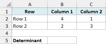
Enter this formula in cell B5 and press Enter:
=MDETERM(B2:C3)
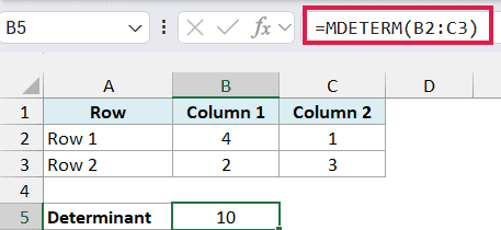
The formula returns 10. For a 2×2 matrix, multiply the top-left number by the bottom-right number, then subtract the product of the other two numbers.
Here, that calculation is 4 × 3 − 1 × 2, which gives 12 − 2 = 10. MDETERM does that calculation for the numbers in B2:C3.
You enter the formula in one cell, even though the input contains several cells. The result is one determinant, so nothing spills into neighboring cells and you don’t need Ctrl+Shift+Enter for this range formula.
Important: A blank cell, text, or a range with unequal row and column counts causes a #VALUE! error. Make sure every matrix entry is numeric; if an entry is zero, enter 0 instead of leaving it blank.
Numbers stored as text also cause this error. If your matrix came from an import, convert those entries to numbers before calculating its determinant.
Example 2: Find a 3×3 Determinant in Excel
The same function handles a larger square matrix without a longer formula.
Below is a three-row matrix on the Three by Three sheet, and I want its determinant in cell B6.
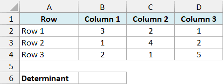
Enter this formula in cell B6:
=MDETERM(B2:D4)
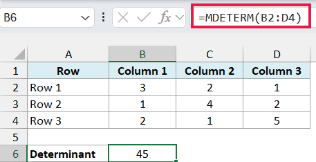
This returns 45. The range B2:D4 includes all nine numbers, and MDETERM calculates one determinant for the whole matrix.
The two-diagonal shortcut from Example 1 applies only to a 2×2 matrix. A 3×3 determinant needs additional multiplication and subtraction, which is why using the function becomes especially helpful as the matrix grows.
For a 4×4 matrix, the approach is the same: select the four rows and four columns of numbers as the array argument. Keep the row and column order intact, because rearranging just one of them can change the determinant’s sign.
Example 3: Understand a Zero Determinant
Sometimes a determinant of zero tells you something useful about the numbers.
Below is a matrix on the Dependent Rows sheet where the second row is twice the first, and I want its determinant in cell B5.
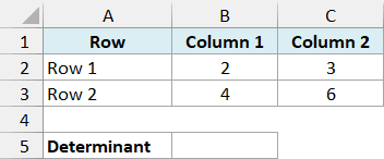
Enter this formula in cell B5:
=MDETERM(B2:C3)
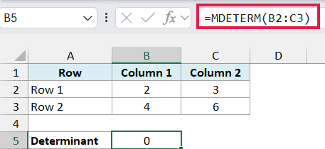
The result is 0, because 2 × 6 − 3 × 4 equals zero. The second row repeats the same relationship at twice the size, so the rows are dependent.
This matrix is called singular, meaning it has no inverse. An inverse is another matrix that reverses the original matrix’s effect when you multiply them together; you can learn more in the MINVERSE function tutorial.
Important: Excel uses finite precision, so a mathematically zero determinant can sometimes appear as a tiny nonzero number. Don’t treat a result such as 1E-16 as reliable proof that a matrix has an inverse.
That notation means 0.0000000000000001. A small determinant can also be a genuine result, so rounding every small value to zero is not a general fix; the scale and precision of your input matter.
Example 4: Choose a Matrix With FILTER
When several matrices share one list, you can select the one you want by its label.
Below are interleaved rows for the Blue and Gold matrices on the Choose a Matrix sheet, and I want the determinant for the label in G1 in cell B9.
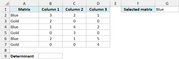
Enter this formula in cell B9:
=MDETERM(FILTER(B2:D7,A2:A7=G1))
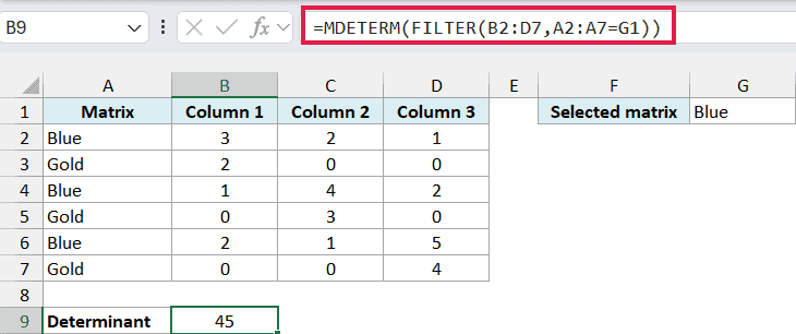
With Blue in G1, the formula returns 45. These are the same nine numbers as the matrix in Example 2, even though Gold rows separate them in this list.
Here is how the formula works:
A2:A7=G1checks which rows have the selected matrix label.- The FILTER function returns the numbers from B2:D7 for those rows, keeping their original order.
- MDETERM calculates the determinant of that three-row, three-column result.
The filtered matrix stays inside the formula. You see only the final determinant in B9, so you don’t need a separate area for the filtered numbers.
Change G1 to Gold and the result becomes 24. Its matrix has 2, 3, and 4 on the main diagonal and zeros everywhere else, so its determinant is their product: 2 × 3 × 4.
Important: Each selected label must return exactly three rows for these three numeric columns. Two or four matching rows produce a non-square array and a #VALUE! error; a label with no matches produces a FILTER #CALC! error.
This combination needs Excel for Microsoft 365, Excel 2024, or Excel 2021. In older Excel versions, copy the chosen matrix’s numeric rows into a separate square range and use MDETERM on that range, as in Example 2.
So these are four ways to work with the MDETERM function in Excel, from a small matrix you can check by hand to a matrix selected from a larger list. I hope you found this tutorial helpful.
Other Excel Articles You May Also Like:
