

The TBILLEQ function in Excel converts a Treasury bill’s discount rate into its bond-equivalent yield. That’s the yearly return you actually earn on the money you pay for the bill.
T-bill rates are quoted as discount rates, and a discount rate always looks a bit lower than what the bill really pays. TBILLEQ gives you a number you can line up against a bond yield, or against another T-bill with a different term.
Unlike most Excel functions, TBILLEQ won’t take whole columns of dates and rates as they are, so plain ranges give you a #VALUE! error. Example 2 shows the one-character fix.
Follow along with the example file
TBILLEQ Function Examples.xlsx
TBILLEQ Function Syntax
Here is the syntax of the TBILLEQ function:
=TBILLEQ(settlement,maturity,discount)
- settlement – the date you buy the T-bill. This is the date it’s traded to you, which comes after the bill’s issue date.
- maturity – the date the T-bill matures and pays you its face value.
- discount – the T-bill’s discount rate, entered as a percentage (3.92%) or a decimal (0.0392).
All three arguments are required. Unlike many of Excel’s bond functions, TBILLEQ has no basis argument, because it always counts the actual days between the two dates.
The maturity date has to be after the settlement date and no more than one year after it. If it isn’t, or if the discount rate is 0 or less, TBILLEQ returns the #NUM! error.
The dates should be real dates in cells, or dates built with the DATE function. If a date can’t be read as a date, TBILLEQ returns the #VALUE! error.
The TBILLEQ function works in Excel 365, 2024, 2021, 2019, and 2016 on Windows, and in Excel 365, 2024, and 2021 for Mac.
When to Use the TBILLEQ Function
Use this function when you need to:
- Turn a T-bill’s quoted discount rate into the yield you actually earn
- Get the yield for a whole list of T-bills with one formula
- Work out the yield when you only know the bill’s term in weeks
- Compare T-bills with different terms on the same footing
- Check how a T-bill stacks up against a bond or another yearly yield
Let me show you a few practical examples of how to use the TBILLEQ function.
Example 1: Convert a T-Bill Discount Rate to Bond-Equivalent Yield
Let’s start with a simple example.
Below are the details of a 13-week T-bill quoted at a 3.920% discount rate, and I want its bond-equivalent yield in cell B6.
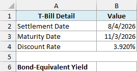
Here is the formula:
=TBILLEQ(B2,B3,B4)
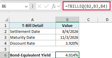
The formula returns 4.014%, which is a bit higher than the 3.920% discount rate.
That’s because the two rates measure the same bill differently. You buy a T-bill for less than its $100 face value and get the full $100 at maturity, and that gap is the discount.
Here, the bill costs about $99.01, so the discount is about $0.99. The discount rate divides that $0.99 by the $100 face value and uses a 360-day year.
The bond-equivalent yield divides the same $0.99 by the $99.01 you actually pay and uses a 365-day year. Over these 91 days, that works out to 4.014% a year.
Example 2: Get the Bond-Equivalent Yield for Several T-Bills at Once
Now let’s say you keep a log of T-bills and want the yield for every one of them.
Below is a list of seven T-bills with their settlement dates, maturity dates, and discount rates, and I want the bond-equivalent yield for each bill in column E.
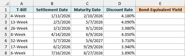
Here is the formula:
=TBILLEQ(+B2:B8,+C2:C8,+D2:D8)
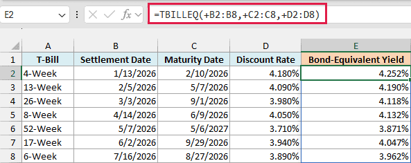
This one formula spills all seven yields into E2:E8.
The plus sign (+) in front of each range is what makes this work. With plain ranges, TBILLEQ returns a single #VALUE! error, but the plus sign turns each range into a list of values, so TBILLEQ returns one result for each bill.
This is the same fix that works for other Excel functions that won’t spill, like the EDATE and EOMONTH functions.
Important: Every range needs its own plus sign. If you leave it off even one of them, every row in the result shows #VALUE!.
Also notice that the yield is higher than the discount rate for every bill, and the gap gets bigger as the term gets longer. It’s 0.072% on the 4-week bill and 0.161% on the 52-week bill.
That happens because a longer bill is sold at a bigger discount, so you pay less up front for the same $100 at maturity.
If you are using Excel 2019 or earlier, enter the below formula in cell E2 and then copy it down the range:
=TBILLEQ(B2,C2,D2)
Example 3: Use the Term in Weeks Instead of a Maturity Date
T-bills are sold by term (4 weeks, 13 weeks, 26 weeks, and so on), so you may know the term rather than the exact maturity date.
Below are the details of a 26-week T-bill, and I want its bond-equivalent yield in cell B6 using the term in B3.
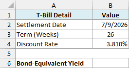
Here is the formula:
=TBILLEQ(B2,B2+B3*7,B4)
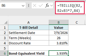
The formula returns 3.939%.
Here, B3*7 turns the 26 weeks into 182 days, and adding that to the settlement date in B2 gives the maturity date (January 7, 2027). This works because Excel stores dates as numbers, one for each day.
Example 4: Rank T-Bills by Bond-Equivalent Yield
Because TBILLEQ puts every bill on the same yearly footing, you can use it to compare T-bills with different terms and see which one pays the most.
Below are this week’s T-bill offerings, all settling on October 1, 2026, and I want them sorted from the highest bond-equivalent yield to the lowest in columns F to H.
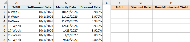
Here is the formula:
=SORT(HSTACK(A2:A8,D2:D8,TBILLEQ(+B2:B8,+C2:C8,+D2:D8)),3,-1)
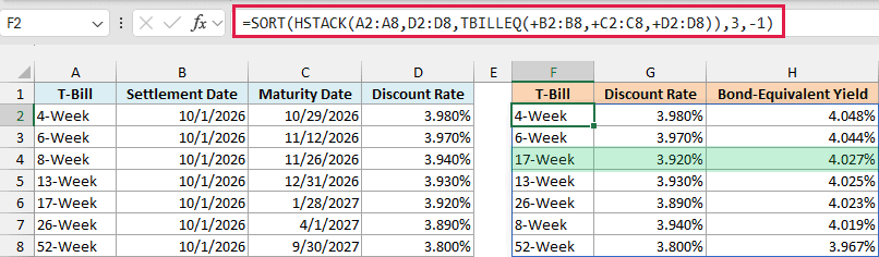
How this formula works:
- TBILLEQ(+B2:B8,+C2:C8,+D2:D8) gets the yield for all seven bills, using the same plus-sign trick from Example 2.
- The HSTACK function puts the bill names, the discount rates, and these yields side by side as one three-column table.
- The SORT function sorts that table by its third column (the yield), and -1 makes it go from highest to lowest.
Now look at the 17-Week bill. Its discount rate (3.920%) is lower than the 13-Week and 8-Week bills, but its yield (4.027%) is higher than both.
The 8-Week bill drops from third place by discount rate to sixth place by yield. So if you pick bills by the quoted discount rate alone, you can end up with the one that pays less.
The HSTACK function is only available in Excel 365 and Excel 2024. If you are using an older version, enter the below formula in cell E2 and then copy it down to E8:
=TBILLEQ(B2,C2,D2)
Then sort A1:E8 by column E (largest to smallest) with the Sort option in the Data tab.
Example 5: The Bond-Equivalent Yield Formula (and Where It Stops Matching)
You might want to see the math behind TBILLEQ, or check its result by hand.
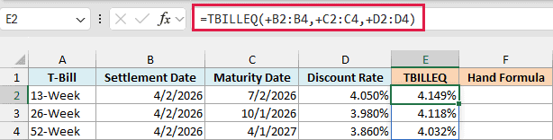
Below are three T-bills with terms of 13, 26, and 52 weeks, and I want the TBILLEQ result in column E and the hand-written formula’s result in column F.

Here is the TBILLEQ formula:
=TBILLEQ(+B2:B4,+C2:C4,+D2:D4)
And here is the bond-equivalent yield formula from Microsoft’s TBILLEQ help page, typed out by hand:
=365*D2:D4/(360-D2:D4*(C2:C4-B2:B4))
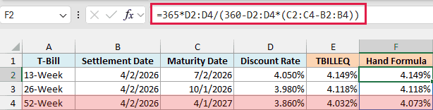
How this formula works (using the 13-week bill, 4.050% for 91 days):
- C2:C4-B2:B4 gives the number of days each bill runs (91, 182, and 364).
- D2:D4*(C2:C4-B2:B4) multiplies the discount rate by the days. For the 13-week bill, that’s 3.6855, and 3.6855 divided by 360 is about 0.0102, which is the $1.02 discount on each $100.
- Subtracting that from 360 gives 356.3145, and 356.3145 divided by 360 is about 0.9898, so you pay about $98.98 for each $100.
- 365*D2:D4 divided by 356.3145 then gives the discount as a share of the price you pay, on a 365-day year, just like in Example 1. The two divide-by-360 steps cancel each other out, which is why the formula doesn’t show them.
For the 13-week and 26-week bills, both columns match exactly (4.149% and 4.118%). For the 52-week bill, they don’t: TBILLEQ gives 4.032%, while the hand formula gives 4.073%.
That’s because the simple formula only applies to bills of 182 days or less. For anything longer, TBILLEQ switches to a longer calculation that matches how a bond pays interest twice a year, and Microsoft’s help page doesn’t show that version.
So use the hand formula only to understand what TBILLEQ does. For the actual yield, especially on bills longer than 26 weeks, use TBILLEQ.
Example 6: Fix the #NUM! Error and Wrong Yields in TBILLEQ
TBILLEQ is strict about its inputs, and a small mistake in the data either gives you an error or a yield that makes no sense.
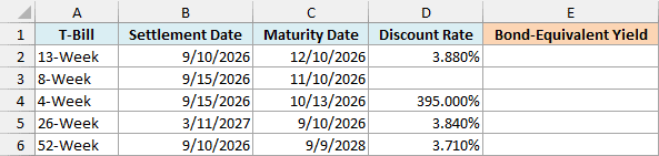
Below is a list of five T-bills where four of them have a mistake in the data, and I want the bond-equivalent yield for each one in column E.
Here is the formula:
=TBILLEQ(+B2:B6,+C2:C6,+D2:D6)
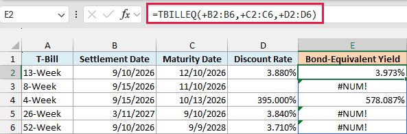
Only the 13-Week bill in row 2 gives a sensible yield (3.973%). Here is what went wrong with the rest:
- In row 3 (8-Week), the discount rate is missing. TBILLEQ treats the blank cell as 0, and a discount rate of 0 or less gives #NUM!.
- In row 4 (4-Week), the rate was entered as 3.95 instead of 3.95%, so Excel reads it as 395%. There’s no error here, just an impossible yield of 578.087%.
- In row 5 (26-Week), the settlement and maturity dates are swapped, so the maturity date comes before the settlement date, which gives #NUM!.
- In row 6 (52-Week), the maturity year was typed as 2028 instead of 2027, which puts maturity two years after settlement. TBILLEQ only works up to one year, so you get #NUM!.
Important: A rate typed as 3.95 instead of 3.95% is 100 times too big, but TBILLEQ shows no error, so it’s easy to miss. If the rate column is formatted as a percentage (as it is here), the mistake shows up as 395.000% in D4.
Once you fix the data (add the 8-Week rate, change 3.95 to 3.95%, swap the 26-Week dates, and correct the 52-Week year to 2027), all five rows return a proper yield.
So these are six practical ways to use the TBILLEQ function in Excel. It turns a T-bill’s discount rate into the yield you actually earn, handles a whole list of bills with one formula, and helps you compare bills with different terms.
If you need the price of a T-bill from its discount rate, use the TBILLPRICE function.
If you know the price, the TBILLYIELD function gives you a yield on a 360-day year, so it comes out a little lower than TBILLEQ.
To get TBILLEQ’s 365-day yield from the price instead, use the INTRATE function with the price, 100 as the redemption, and basis 3 (for bills of 26 weeks or less).
I hope you found this Excel tutorial useful.
Other Excel Articles You May Also Like:
