

The BESSELI function in Excel returns the modified Bessel function In(x) for a value x and an order n. It turns up in engineering and physics formulas, and in signal processing.
Think of In(x) as a family of curves. The order n picks the curve, and x is the point along it where you read the value.
At x = 0, the order-0 curve sits at exactly 1 and every higher order sits at 0. From there each curve climbs very quickly as x gets bigger.
One thing to watch for: if you give BESSELI a range of cells directly, it returns #VALUE! instead of spilling. A leading + in front of the range fixes it, and the examples below use it.
In this tutorial, I’ll show you how to calculate BESSELI values, compare orders, handle bad inputs, check the result against its own series, and use it in a seasonal sales model.
Follow along with the example file
BESSELI Function Examples.xlsx
BESSELI Function Syntax
Here is the syntax of the BESSELI function:
=BESSELI(x, n)
- x is required. It is the number at which you want to evaluate the function, and it can be negative.
- n is required. It is the order of the function, which picks which curve in the family you want: 0, 1, 2, and so on.
Leaving out the order makes Excel reject the formula, and an empty argument, such as =BESSELI(1,), returns #N/A.
If n isn’t a whole number, Excel drops the decimal part instead of rounding it, so an order of 1.9 is treated as 1.
BESSELI is available in Excel for Microsoft 365, 2024, 2021, 2019, and 2016, including supported Mac editions. The spilling examples below use dynamic-array Excel, such as Microsoft 365, 2024, or 2021; single-cell alternatives are included for older versions.
When to Use the BESSELI Function
Use the BESSELI function when you need to:
- Evaluate the modified Bessel function In(x) inside an engineering or physics formula.
- Compare how In(x) changes from one order to the next.
- Scale a wrap-around pattern, such as months of the year or hours of the day, so its shares add up to 100%.
- Check a hand-built calculation of In(x) against Excel.
The workbook has one sheet for each example, named Example 1 through Example 5. Let’s start with a plain list of x values.
Example 1: Calculate Order-0 Values for a List of x
Let’s start with the simplest case, a single order applied to a whole list.
Below is a list of x values from 0 to 8, and I want the order-0 modified Bessel function for each one in column B.
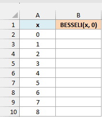
Enter this formula in cell B2 and press Enter:
=BESSELI(+A2:A10,0)
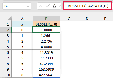
The formula returns nine results, spilling from B2 down to B10. For x = 0 the result is exactly 1, and for x = 1 it is about 1.2661.
Notice how fast the numbers grow. By x = 8 the result is already about 427.56, and the values never turn back down or go negative.
The + before A2:A10 makes Excel pass the values in the range as an array. It doesn’t change any of the numbers.
Important: Keep the leading + in range-based formulas. Without it, BESSELI returns #VALUE! when you give it a range, even in dynamic-array Excel.
Make sure B2:B10 is empty before you enter the formula. If something is already there, Excel returns #SPILL!.
The workbook shows four decimal places, but the cells keep the full result.
If you are using Excel 2019 or earlier, enter the below formula in cell B2 and then copy it down to B10:
=BESSELI(A2,0)
Example 2: Compare Orders 0 to 3 Side by Side
Now let’s compare several orders at once.
Below are x values from 0 to 5 and the orders 0 to 3, and I want the BESSELI result for every x and order pair, starting in column C.
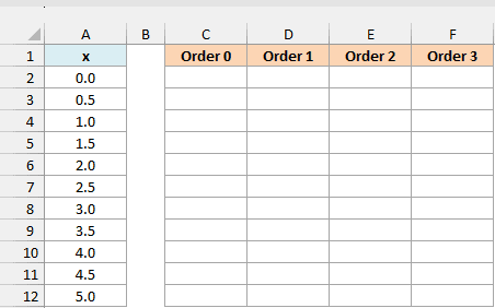
Enter this formula in cell C2:
=BESSELI(+A2:A12,+C1:F1)
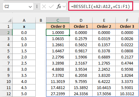
One formula fills the whole grid with 44 results. Excel pairs each x in column A with each order in row 1, which is why both ranges carry a +.
The headers read Order 0 to Order 3, but each one is just the number 0, 1, 2, or 3 with a custom number format. That is what lets the formula use them as the order.
Read down any column and the values climb as x grows. Read across a row and they shrink as the order goes up.
At x = 2, for example, the four orders give about 2.2796, 1.5906, 0.6889, and 0.2127.
At x = 0, the order-0 result is 1 and every higher order is 0.
If you are using Excel 2019 or earlier, enter the below formula in cell C2 and then copy it across to column F and down to row 12:
=BESSELI($A2,C$1)
Example 3: Handle Negative x, Decimal Orders, and Errors
Next, let’s see what BESSELI does with awkward inputs.
Below are pairs of x values and orders, and I want the BESSELI result for each pair in column C.
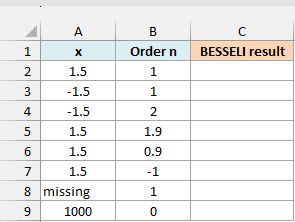
Enter this formula in cell C2:
=BESSELI(+A2:A9,+B2:B9)
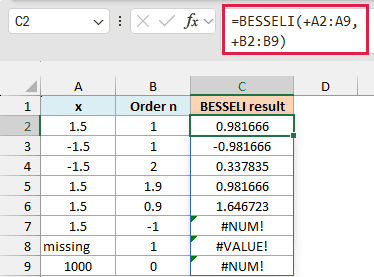
Start with the first three rows. At order 1, x = 1.5 gives 0.981666 and x = -1.5 gives -0.981666, so an odd order flips the sign.
At order 2, x = -1.5 gives a positive 0.337835, the same as x = 1.5 at order 2 in Example 2. Even orders return the same result for x and -x.
Rows 5 and 6 show what happens to a decimal order. An order of 1.9 is treated as 1, so row 5 matches row 2.
An order of 0.9 is treated as 0, so row 6 returns the order-0 result for 1.5, which is 1.646723.
The last three rows return errors on purpose. A negative order, like the -1 in row 7, returns #NUM!.
That holds even for a decimal such as -0.5, which would otherwise drop to 0.
Row 8 has the text “missing” in the x column, so it returns #VALUE!. Replace the text with a number to fix it.
Row 9 uses x = 1000, which returns #NUM! because the calculation overflows Excel’s number range. For order 0, that happens somewhere between x = 705 and x = 710.
If you are using Excel 2019 or earlier, enter the below formula in cell C2 and then copy it down to C9:
=BESSELI(A2,B2)
Example 4: Check BESSELI Against Its Series
The number BESSELI returns is the sum of an endless series of terms, and you can build that sum yourself to see where it comes from.
For order n, each term is (x/2)^(2k+n) divided by the product of k! and (k+n)!, where k counts 0, 1, 2, and so on. The ! means factorial: k! is 1 x 2 x … x k (with 0! defined as 1), which the FACT function calculates.
For x = 2 and order 1, the terms shrink quickly once k grows, so eight terms are plenty. A larger x needs more terms.
Below is a list of k values from 0 to 7, with x = 2 and the order n = 1 in a small table beside it, and I want the series term for each k in column B.
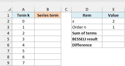
Enter this formula in cell B2:
=(E2/2)^(2*A2:A9+E3)/(FACT(A2:A9)*FACT(A2:A9+E3))
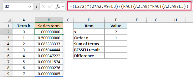
Here is how the formula works:
(E2/2)^(2*A2:A9+E3)is the top of each term. E2 holds x, E3 holds the order, and A2:A9 holds k.FACT(A2:A9)*FACT(A2:A9+E3)is the bottom of each term, the product of k! and (k+n)!.
The first term is 1 and the second is 0.5. By k = 7, the term is only about 0.000000005, and the next one would be about 0.00000000007.
The FACT function accepts the range directly, and the arithmetic in the formula already turns the range into an array, so this formula doesn’t need a +.
Enter this formula in cell E4 to add up the terms:
=SUM(B2:B9)
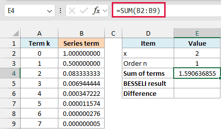
Now enter this formula in cell E5 to get the same value from BESSELI:
=BESSELI(E2,E3)
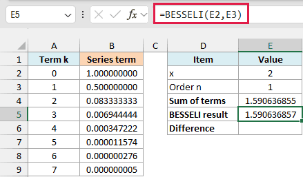
Both results round to 1.5906369 at seven decimal places. Enter this formula in cell E6 to see how far apart they are:
=E4-E5
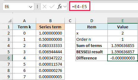
The difference is about -0.000000003, which is in the ninth decimal place. The eight terms are accurate to about ten decimal places, so the gap comes from BESSELI.
Important: BESSELI is an approximation, so trust its results to about seven significant digits. Don’t compare them to another source with an equals sign, because the last digits will rarely match.
Compared with exact values calculated independently, the largest relative difference across the BESSELI results in this workbook was about 2.5 in 100 million. That is plenty for most practical uses.
If you are using Excel 2019 or earlier, enter the below formula in cell B2 and then copy it down to B9:
=($E$2/2)^(2*A2+$E$3)/(FACT(A2)*FACT(A2+$E$3))
Example 5: Build a Seasonal Sales Model with BESSELI
Here is a practical use for BESSELI. Some patterns wrap around, like the months of the year, where December sits right next to January.
A smooth curve for that kind of pattern is called the von Mises distribution, and BESSELI supplies the number that makes it add up to 100%.
Below are the months numbered 1 to 12, with the peak month in E2 and the concentration in E3, and I want the share of an ice cream stand’s annual sales for each month in column B.
The inputs are made up for the model; they aren’t real sales data.
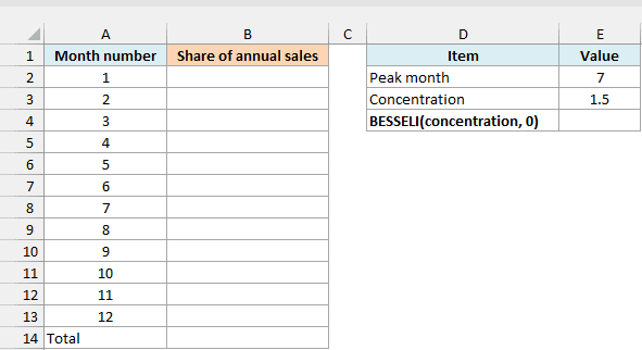
The peak month is 7, which means July. The concentration is 1.5, and it controls how sharply sales pile up around that peak (statisticians call it kappa).
First, enter this formula in cell E4 to get the scaling number:
=BESSELI(E3,0)
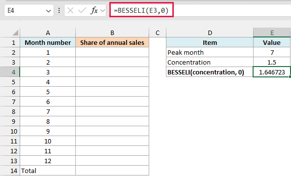
It returns about 1.646723. This is the order-0 result for the concentration of 1.5.
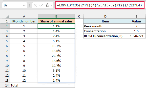
Now enter this formula in cell B2:
=EXP(E3*COS(2*PI()*(A2:A13-E2)/12))/(12*E4)
Here is how the formula works:
2*PI()*(A2:A13-E2)/12turns each month’s distance from the peak into an angle on a circle, where 12 months make one full turn.- The COS function returns 1 at the peak month and -1 six months away.
- The EXP function and the concentration in E3 turn that into a curve. A bigger concentration makes a sharper peak.
- Dividing by
12*E4scales the results. Twelve months share the curve, and the BESSELI result in E4 is the matching adjustment that makes them add up to 100%.
July gets the biggest share at 22.7%, and January, six months away, gets the smallest at 1.1%. December and February both come out at 1.4%, because each is five months from July, one on either side.
To confirm the shares add up, enter this formula in cell B14:
=SUM(B2:B13)
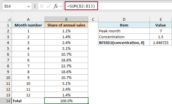
The total is 100.0%. If you divided by 12 alone, the shares would add up to about 165%, and the BESSELI result is what brings the total back to 100%.
Pro Tip: Change the concentration in E3 to reshape the curve: 0 gives every month 8.3%, and larger values pile more sales around the peak. The total stays at 100.0% up to 5 but reaches about 100.2% at 10.
If you are using Excel 2019 or earlier, enter the below formula in cell B2 and then copy it down to B13:
=EXP($E$3*COS(2*PI()*(A2-$E$2)/12))/(12*$E$4)
So these are five ways to use BESSELI, from a simple list of values to a seasonal model. Excel also has BESSELJ, BESSELK, and BESSELY for the other Bessel functions.
I hope you found this tutorial helpful.
Other Excel Articles You May Also Like:
