

The BESSELK function in Excel returns the modified Bessel function of the second kind, written Kn(x). The x is the point where you want the value, and the n is the order, which picks which version of the function you get.
Every version starts very large when x is close to zero and drops toward zero quickly as x gets bigger. You will mostly meet it in physics and engineering formulas for things that fade out fast, such as heat flowing through a round fin.
You don’t need to know the math behind it to use the function. You give BESSELK an x and an order, and it returns the value.
In this article, I’ll show you how to use BESSELK with five examples. BESSELK won’t take a range of cells directly, so filling a whole column with one formula needs a small trick.
Follow along with the example file
BESSELK Function Examples.xlsx
BESSELK Function Syntax
Here is the syntax of the BESSELK function:
=BESSELK(x, n)
- x – The value at which you want to evaluate the function. It has to be greater than zero.
- n – The order of the function (the n in Kn(x)), such as 0, 1, 2, and so on. It picks which version of the function you get, and it can’t be negative.
The x value must be above zero, because the curve climbs without limit as x gets close to zero. If x is zero or negative, BESSELK returns the #NUM! error.
For n, order 0 is the lowest order, and each higher order gives a larger value at the same x. If n has a decimal part, Excel drops it instead of rounding, so =BESSELK(2,1.9) gives the same result as =BESSELK(2,1).
The BESSELK function works in Excel for Microsoft 365, Excel 2024, 2021, 2019, 2016, and Excel for Mac. The single formulas that fill a whole column or grid need Excel 365 or Excel 2021 and later.
When to Use the BESSELK Function
Use this function when you need to:
- Get the value of the modified Bessel function Kn(x) without looking it up in a math table
- Work through physics or engineering formulas where an effect fades quickly with distance
- Build a table of Kn(x) values for several orders and x values
- Check hand calculations or results from other software against the same function
Let me show you a few practical examples of how to use the BESSELK function.
Example 1: Get BESSELK Values for Different x and Orders
Let’s start with a simple example.
Below is a list of x values with the order I want for each one, and I want the BESSELK result in column C.
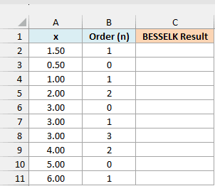
Here is the formula to enter in cell C2 and copy down:
=BESSELK(A2,B2)
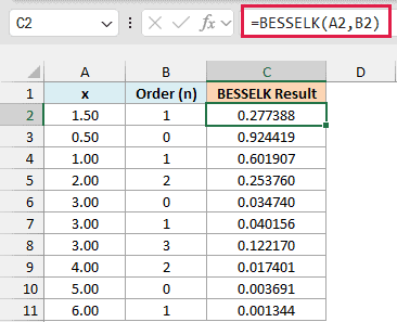
BESSELK takes the x value from column A and the order from column B, and returns the value of that Bessel function. The first row (x of 1.5 and order 1) is the sample from Microsoft’s own help page, which gives about 0.277388.
For the same order, a bigger x gives a smaller value, so order 0 drops from 0.924419 at x of 0.5 to 0.003691 at x of 5.
And for the same x, a higher order gives a bigger value. At x of 3, order 0 gives 0.034740, order 1 gives 0.040156, and order 3 gives 0.122170.
Excel’s BESSELK values are accurate to about seven significant digits, because the function uses an approximation. For x of 2 and order 2, it returns 0.25375976, while a more precise value from a math library is 0.2537597546.
The difference is tiny, but don’t expect the last digits to match another tool.
I’ve kept this first example as a per-row formula so you can see how BESSELK works on one pair at a time. The next example fills a whole column with one formula.
Example 2: Fill a Whole Column with One BESSELK Formula
In Excel 365 (and Excel 2021 or later), you can get all the values with a single formula, but BESSELK needs a small trick to do it.
Below is a list of x values (think of x as the distance from a source), and I want the K0 value for each one in column B.
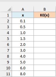
The K0 here means order 0, so the n in the formula is 0 for every row. Here is the formula to enter in cell B2:
=BESSELK(+A2:A11,0)
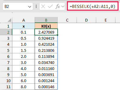
This spills the results down to B11, with one value for each x.
You can see the decay in the numbers. The value is 2.427069 at x of 0.1, 0.421024 at x of 1, and only 0.000146 at x of 8.
The plus sign in front of the range is the important part. Without it, BESSELK returns a single #VALUE! error instead of ten results.
Here’s what that looks like. I’ve entered the same formula without the plus sign in cell D2:
=BESSELK(A2:A11,0)
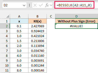
This happens because BESSELK can’t take a multi-cell range reference like A2:A11. It only works with single values, or with a list of values held in memory (called an array).
Putting a plus sign in front of a range makes Excel hand BESSELK its values as an array, so it returns one result for each row.
The COMPLEX function has the same quirk, and the same plus sign fixes it. Since the x values here are numbers, a double minus (--A2:A11) or multiplying by 1 (A2:A11*1) would also work.
If you are using Excel 2019 or earlier, enter the below formula in cell B2 and then copy it down the range:
=BESSELK(A2,0)
Example 3: Build a Table of BESSELK Values for Several Orders
Now let’s fill a whole grid with one formula.
Below I have a list of x values down the side and the orders 0 to 4 across the top, and I want the BESSELK value for every pair in the grid.
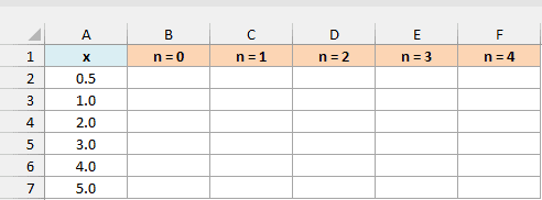
Here is the formula to enter in cell B2:
=BESSELK(+A2:A7,+B1:F1)
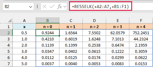
The x values are in a column and the orders are in a row, so Excel pairs every x with every order. That fills the grid from B2 to F7 with one formula.
Both ranges need the plus sign, for the same reason as in the last example.
The headers show “n = 0” and so on, but the cells hold plain numbers (0 to 4), which is what the formula reads. A custom number format adds the “n = ” text on screen only.
Read down any column and the values fall as x grows. Read across any row and they rise with the order, so at x of 0.5 the values climb from 0.9244 at order 0 to 752.2451 at order 4.
If you are using Excel 2019 or earlier, enter the below formula in cell B2 and then copy it across and down the grid:
=BESSELK($A2,B$1)
Example 4: Find Where BESSELK Drops Below a Cutoff
Let’s use the curve to answer a question.
Below is a list of x values in ascending order, and I want to find the first x where K0 drops below the cutoff in cell E2. I’ll start by getting the K0 value for each x in column B.
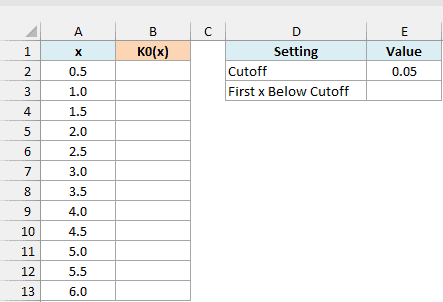
Here is the formula to enter in cell B2:
=BESSELK(+A2:A13,0)
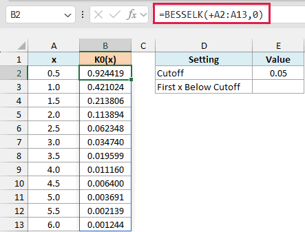
Now I want the first x where that value falls below the cutoff of 0.05. Here is the formula to enter in cell E3:
=XLOOKUP(TRUE,B2:B13<E2,A2:A13)
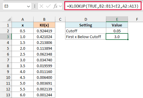
The B2:B13<E2 part checks every K0 value against the cutoff and returns TRUE or FALSE for each row. The XLOOKUP function finds the first TRUE and returns the x value from the same row.
K0 only falls as x grows, so that first TRUE is the first x below the cutoff. The result is 3, because K0 at 2.5 is still 0.062348, and at 3 it drops to 0.034740.
Change the cutoff in E2 to 0.01, and the formula returns 4.5. If no x in the list is below the cutoff, the formula returns #N/A, so extend the list of x values.
If you are using Excel 2019 or earlier, enter the below formula in cell B2 and then copy it down the range:
=BESSELK(A2,0)
And then enter the below formula in cell E3:
=INDEX(A2:A13,MATCH(TRUE,INDEX(B2:B13<E2,0),0))
Example 5: Fix #NUM! and #VALUE! Errors in BESSELK
Let’s look at the inputs that make BESSELK fail, and a couple that work when you might not expect them to.
Below are a few test cases, each with a case name, an x value, and an order, and I want to see what BESSELK returns for each one in column D.
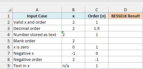
Here is the formula to enter in cell D2 and copy down:
=BESSELK(B2,C2)
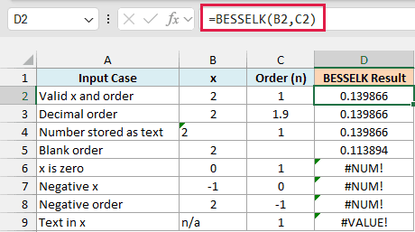
The first case (x of 2 and order 1) works as expected and returns about 0.139866. In the Decimal order case, the order of 1.9 is truncated to 1, so the result is the same 0.139866 (it is not rounded up to 2).
The Number stored as text case also works, even though its 2 is text (it sits on the left side of the cell). BESSELK converts a number stored as text into a real number, so you don’t have to fix it first.
The x is zero, Negative x, and Negative order cases return the #NUM! error. An x of zero or a negative x fails because x has to be above zero, and a negative order fails because the order can’t be negative.
The Text in x case holds the text n/a, so it returns #VALUE!. Text that can’t be read as a number fails, while text that looks like a number, such as the 2 above, gets converted.
Important: A blank order doesn’t give an error. In the Blank order case, BESSELK treats the empty cell as 0 and returns the K0 value, so a missing order can quietly look like a valid result.
So these are some practical ways to use the BESSELK function in Excel to get values of the modified Bessel function.
Just remember that x has to be above zero, and put a plus sign in front of your ranges when you want one formula for a whole column or grid. I hope you found this article helpful.
Other Excel Articles You May Also Like:
