

The CUBERANKEDMEMBER function returns the item at a position you choose from a sorted list, such as the first, second, or third one. Use it to build a top 3 or bottom 3 list that updates with your data.
It works with the Data Model, which is a table stored inside the workbook, and not with a plain range of cells. The example file you can download already has a working Data Model, so you don’t have to connect to anything to follow along.
In this tutorial, I’ll show you how to find the top reader, build a top 3 list with one formula, and see why the list needs a sort order. You’ll also get the bottom 3, add a caption, and handle a rank that’s too high.
Follow along with the example file
CUBERANKEDMEMBER Function Examples.xlsx
CUBERANKEDMEMBER Function Syntax
Here is the syntax of the CUBERANKEDMEMBER function:
=CUBERANKEDMEMBER(connection, set_expression, rank, )
In cube terms, a set is a list of items, such as every reader in a table, and a member is one item in that list, such as one reader.
- connection is the name of the data connection, entered in double quotes. The Data Model inside a workbook is named
ThisWorkbookDataModel, and a cube on a server has its own connection name. - set_expression is the set you want to pick from. It is usually a cell that holds a CUBESET formula, but you can also write the CUBESET formula directly inside.
- rank is the position you want, where 1 is the first member of the set, 2 is the second, and so on.
- caption is optional text that Excel shows in the cell instead of the member’s own name.
CUBERANKEDMEMBER doesn’t sort anything. It counts to the position you ask for in the set, so the order of the set decides what “first” means.
The sorting therefore happens in the CUBESET formula that builds the set, which you’ll see in the first example.
I tested these examples in Excel for Microsoft 365 on Windows (build 20618). I haven’t tested them on Mac, Excel on the web, or with a server cube.
When to Use the CUBERANKEDMEMBER Function
Use this function when you need to:
- Show the top or bottom few items from a Data Model, such as the best-selling products
- Build a leaderboard that refreshes when the model’s data changes
- Pull one specific position, like third place, into a report cell
- Feed a ranked item to another cube function, such as CUBEVALUE, to show its total
If your data is just a list on a worksheet, a regular formula such as the SORTBY function is simpler. CUBERANKEDMEMBER earns its place when the totals you rank already live in a Data Model.
Let me show you how it works with the reading challenge data in the example file.
Example 1: Find the Top Reader
Let’s start with the simplest case, finding the reader who finished the most books.
Below is a reading challenge log with the books each reader finished in each genre, and I want to find the top reader in cell F3.
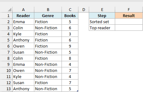
The log is a table named Reading, and it’s already in the workbook’s Data Model. The model also has a measure named Total Books that adds up the Books column, so each reader’s total comes from both of their rows.
First, enter this CUBESET formula in cell F2 to line up the readers from most books to fewest:
=CUBESET("ThisWorkbookDataModel","[Reading].[Reader].[Reader].Members","Top readers",2,"[Measures].[Total Books]")
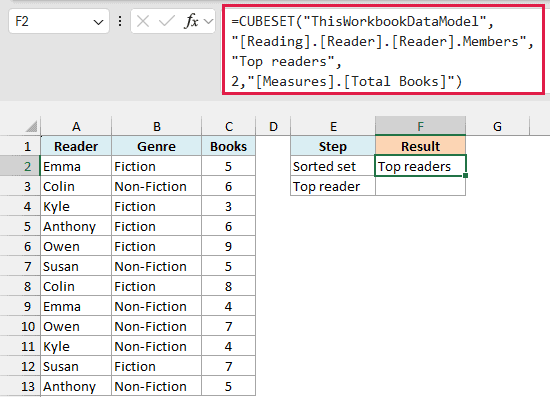
Here is how this formula works:
[Reading].[Reader].[Reader].Membersis every reader in the table. Reading is the table and Reader is its column, and the name appears twice because the model has a field and a level that are both called Reader."Top readers"is the caption the cell displays.2sorts the set in descending order.[Measures].[Total Books]is the measure to sort by.
The cell only shows the caption. The sorted list of readers is stored behind it, ready for the next formula to read.
Now enter this formula in cell F3:
=CUBERANKEDMEMBER("ThisWorkbookDataModel",F2,1)
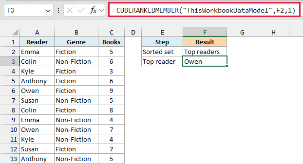
The result is Owen, who finished 16 books, 9 fiction and 7 non-fiction. That’s more than anyone else.
The formula asks the set in F2 for its first member. Because the set is sorted from most books to fewest, the first member is the top reader.
You can also write the CUBESET formula directly in the second argument, but keeping it in its own cell lets several formulas share one set.
Example 2: Build a Top 3 List With One Formula
Now let’s turn that into a top 3 list, without writing three separate formulas.
Below I have the same sorted set in cell B2 and the ranks 1 to 3 in column A, and I want the reader for each rank in column B.
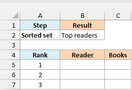
Here is the formula:
=CUBERANKEDMEMBER("ThisWorkbookDataModel",B2,A5:A7)
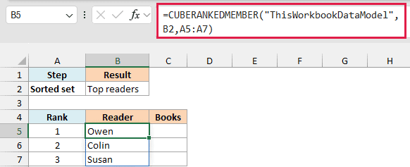
This returns Owen, Colin, and Susan.
The rank argument points at A5:A7 instead of a single number, so the formula returns one member for each rank and spills down automatically. Type 1 to 3 in column A and you get the top three readers.
Next, I want the number of books beside each name in column C. Enter this formula in cell C5 and copy it down to C7:
=CUBEVALUE("ThisWorkbookDataModel","[Measures].[Total Books]",B5)
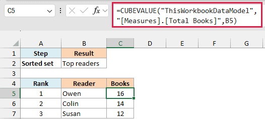
CUBEVALUE looks up the Total Books measure for the reader in B5, which gives 16, 14, and 12. This one stays a per-row formula because, in my test, giving CUBEVALUE the whole spilled range returned #N/A.
If you are using Excel 2019 or earlier, enter the below formula in cell B5 and then copy it down the range, since those versions can’t spill:
=CUBERANKEDMEMBER("ThisWorkbookDataModel",$B$2,A5)
Pro Tip: You can skip the rank column by replacing A5:A7 with SEQUENCE(3), which produces 1, 2, and 3. A bigger number gives a longer list.
Example 3: Why the Set Needs a Sort Order
So far the set has always been sorted. Let’s see what happens when it isn’t.
Below I have the ranks 1 to 3 in column A, and I want the first three readers from the full reader list in column B.
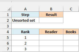
First, enter this CUBESET formula in cell B2, which is the same as before without the last two arguments:
=CUBESET("ThisWorkbookDataModel","[Reading].[Reader].[Reader].Members","All readers")
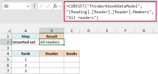
Then enter this formula in cell B5 to ask for the ranks in A5:A7:
=CUBERANKEDMEMBER("ThisWorkbookDataModel",B2,A5:A7)
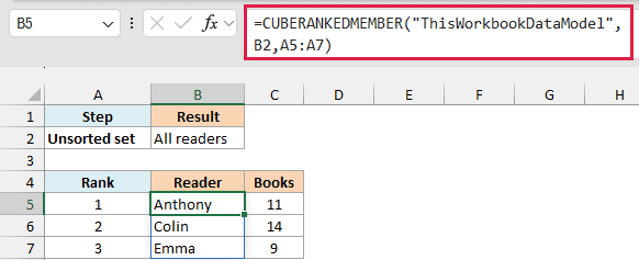
The result is Anthony, Colin, and Emma. I’ve also copied the CUBEVALUE formula from Example 2 into C5:C7, and it shows they read 11, 14, and 9 books.
Without a sort order, rank 1 is simply whoever comes first in the set. In this model that’s alphabetical order, not the order of the rows in the table (Emma is the first row) and not the order of books read.
Important: Always sort the CUBESET when “first” should mean top or bottom. An unsorted set still returns names without any error, so you won’t notice that the top reader is wrong.
Example 4: Get the Bottom 3 Readers
To flip the list, you only need to flip the sort order.
Below I have the ranks 1 to 3 in column A, and I want the three readers who finished the fewest books in column B.
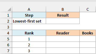
Enter this CUBESET formula in cell B2:
=CUBESET("ThisWorkbookDataModel","[Reading].[Reader].[Reader].Members","Lowest readers",1,"[Measures].[Total Books]")
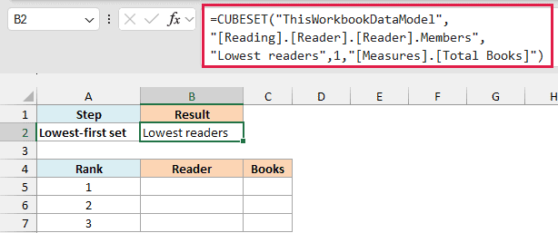
The sort order is now 1, which sorts from the fewest books to the most. Now enter this formula in cell B5 to ask for the ranks in A5:A7:
=CUBERANKEDMEMBER("ThisWorkbookDataModel",B2,A5:A7)
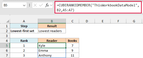
This returns Kyle, Emma, and Anthony. The CUBEVALUE formula in C5:C7 shows they read 7, 9, and 11 books.
The rank formula didn’t change at all. Because the set now starts with the lowest total, rank 1 is the bottom reader.
Pro Tip: To get the last member of a set, use the CUBESETCOUNT function as the rank, as in CUBESETCOUNT(B2). It returns the number of members, so here it points at the sixth and final reader, who is Owen.
Example 5: Show a Custom Caption
The fourth argument lets you show your own label instead of the member’s name.
Below I have the sorted set in cell B2, and I want to show the top reader under the label Reading champion in cell B5.
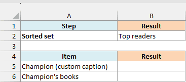
Here is the formula:
=CUBERANKEDMEMBER("ThisWorkbookDataModel",B2,1,"Reading champion")
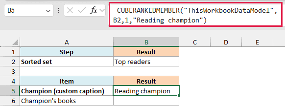
The cell displays Reading champion instead of Owen. The caption only changes what you see, and the cell still holds the member Owen.
To prove that, enter this formula in cell B6:
=CUBEVALUE("ThisWorkbookDataModel","[Measures].[Total Books]",B5)
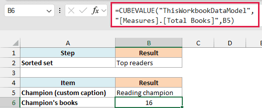
It returns 16, the number of books Owen read. CUBEVALUE uses the member behind B5 and ignores the caption.
Important: Use a caption only in a single-cell formula. If you add one to a formula that spills, every row shows the same caption.
Example 6: Handle a Rank Beyond the Set
Finally, let’s see what happens when you ask for more positions than the set has.
Below I have the sorted set in cell B2 and the ranks 1 to 8 in column A, and I want the reader for each rank in column B. There are only six readers.
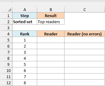
Here is the formula:
=CUBERANKEDMEMBER("ThisWorkbookDataModel",B2,A5:A12)
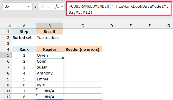
The first six ranks return the readers, and ranks 7 and 8 return #N/A because the set has no seventh or eighth member.
That’s fine on a leaderboard that always has enough members, but it looks messy when a short list leaves errors at the bottom. Enter this formula in cell C5, which wraps the first one in the IFNA function to show a dash instead:
=IFNA(CUBERANKEDMEMBER("ThisWorkbookDataModel",B2,A5:A12),"-")
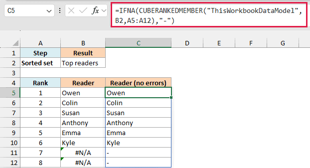
IFNA only replaces #N/A. Unlike the IFERROR function, it doesn’t hide other errors, such as #VALUE! from a rank written as a word, like two.
Important: Microsoft’s page says a wrong connection name returns #NAME?. In my test, a wrong connection, a rank of 0, a negative rank, and a rank beyond the set all returned #N/A.
IFNA hides all of these, so check the connection name and the ranks before you wrap the formula.
That’s how you pull the first, second, or nth item out of a sorted set. The CUBESET decides the order, so sort it before you ask for a rank.
I hope you found this tutorial useful.
Other Excel Articles You May Also Like:
