Connect Slicer to Multiple Pivot Tables in Excel

If you work with Pivot Tables and also use slicers, you may sometimes wonder whether a slicer can be used to control multiple Pivot Tables.

The answer is, of course, YES (otherwise I won’t be writing about it).

This is useful when you have multiple Pivot Tables and you want all of them to update when you make a selection in one slicer.

Instead of having separate slicers for each Pivot Table (which can make your reports look cluttered), you can have one slicer that controls them all.

In this tutorial, I’ll show you exactly how to connect a slicer to multiple pivot tables.

I’ll cover two different scenarios – when your Pivot Tables are created from the same data source (which is super easy), and when they’re created from different data sources (which requires a bit more setup but is still super easy).

Scenario 1: Connecting Slicer to Pivot Tables Made from Same Data Source

This is the easier of the two scenarios.

When you create a Pivot Table using a data source, Excel first creates a Pivot Cache (which is a copy of that data source), and then uses this Pivot Cache to create the Pivot Table. This Pivot Cache is created because it makes using Pivot Tables fast and efficient.

Now, when you create another Pivot Table that uses the same data source, instead of creating a separate Pivot Cache, Excel uses the same Pivot Cache for both the Pivot tables.

This shared cache connection makes it really simple to connect them to the same slicer.

Let me show you how it works with an example.

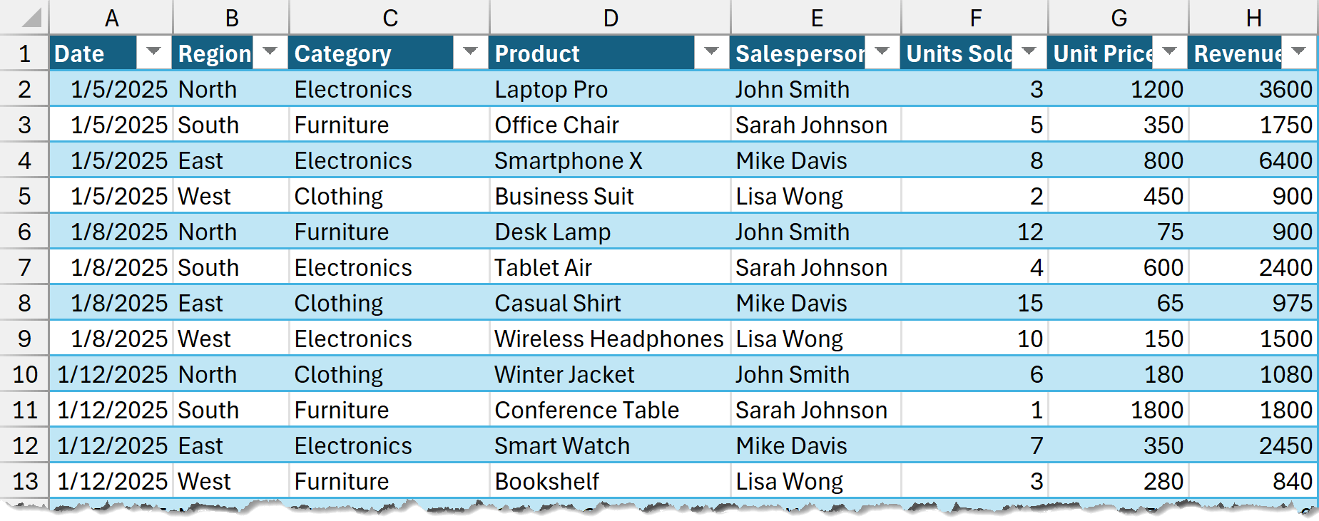
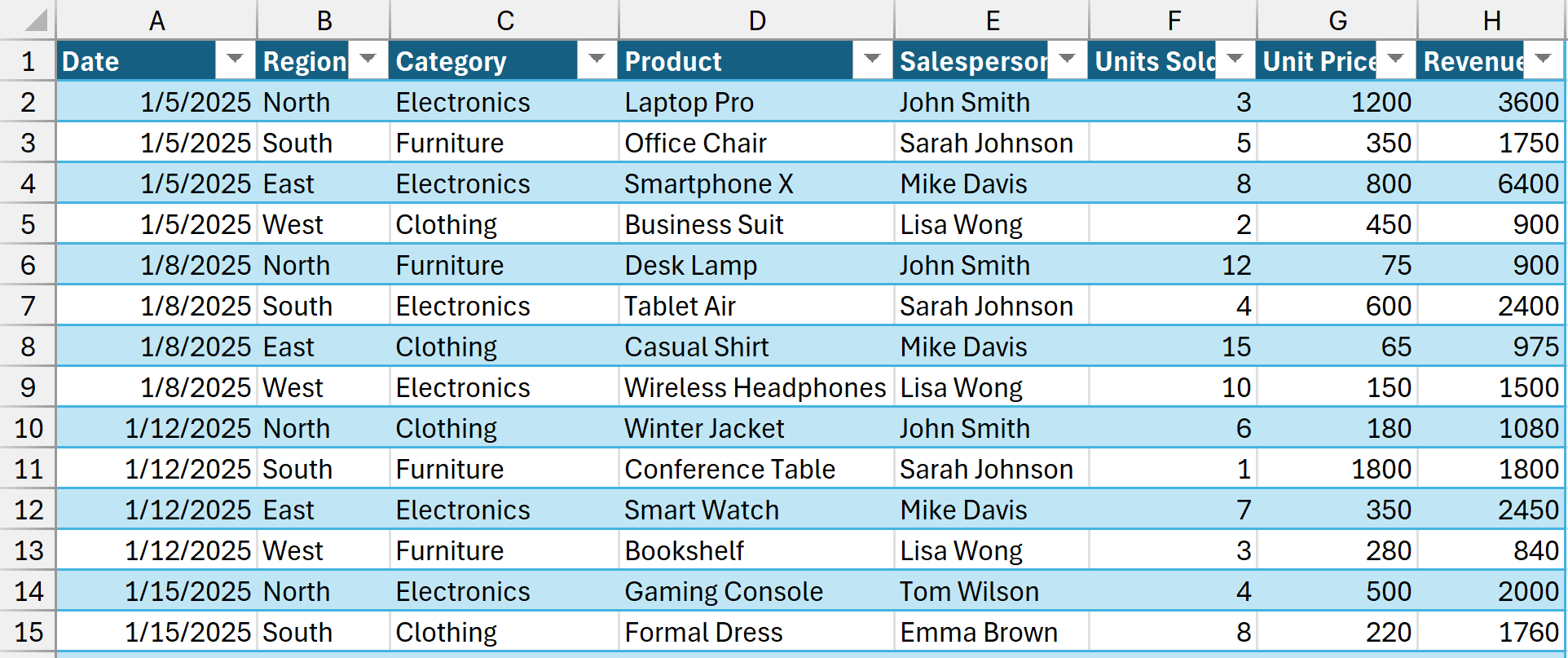
Below I have a sales transaction dataset where I want to create two different pivot tables and then control both with a single slicer.

Step 1 – Creating the First Pivot Table

Here are the steps to create the first Pivot Table:

1. Select any cell in the source data
2. Go to the Insert tab and click on PivotTable (or use the keyboard shortcut Alt + N + V + T). This will open the PivotTable from table or range dialog box

3. In the dialog box, choose New Worksheet

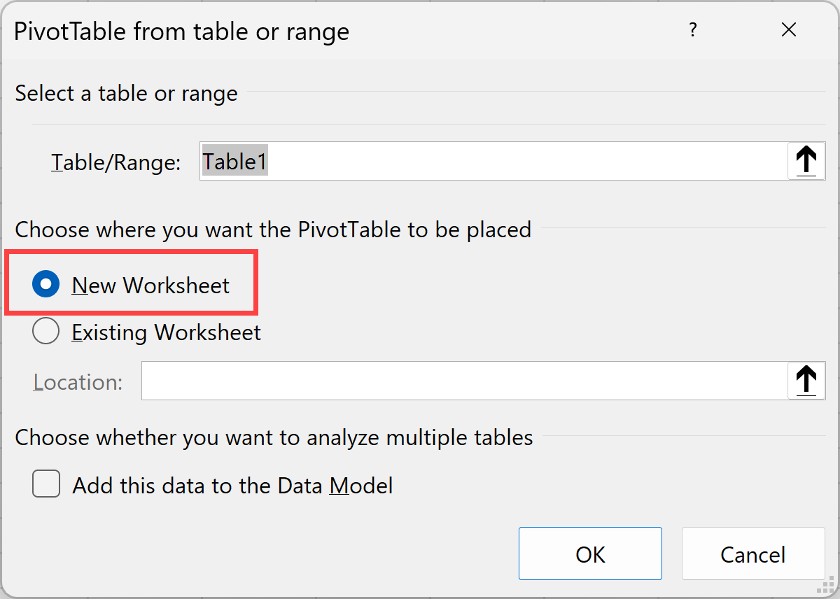
4. Click OK

This will insert a new worksheet and create a blank pivot table in this newly inserted sheet.

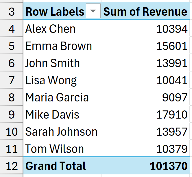
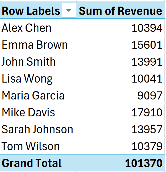
Let’s now configure this Pivot Table by adding ‘Salesperson’ field in the rows area and ‘Revenue’ field in the values area. This will give us a pivot table as shown below.

Step 2 – Creating the Second Pivot Table

Now, for the second pivot table, you have two options:

Option 1: Create from scratch

• Go back to your data source and repeat the same steps we used to create the first Pivot Table
  • Select any cell in the source data
  • Go to the Insert tab and click on PivotTable (or use the keyboard shortcut Alt + N + V + T).
  • In the dialog box, choose New Worksheet
  • Click OK

Option 2: Copy and paste the existing pivot table

• Select the entire first Pivot Table
• Copy it (Ctrl + C)
• Paste it where you want the second pivot table

Note: When you copy and paste a pivot table, it automatically uses the same data source and pivot cache, which is exactly what we want for this technique to work.

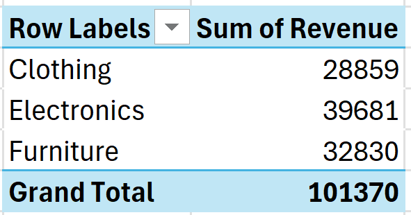
For this example, let’s modify the second pivot table to show revenue by category instead of by salesperson. The second pivot table would look something like this:

Step 3 – Connecting the Slicer to Both Pivot Tables

Now comes the fun part – connecting both Pivot Tables to a single slicer.

To do this, we will first create a slicer for one of the Pivot Tables and then connect the same slicer to the second Pivot Table.

Here are the steps to insert the slicer for the first Pivot Table.

1. Select any cell in the first Pivot Table
2. Go to the PivotTable Analyze tab
3. Click on Insert Slicer

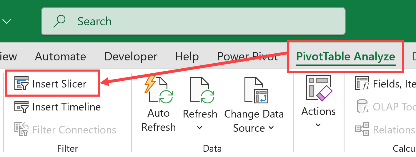
4. Choose the field you want to filter by (let’s choose “Category” for this example)

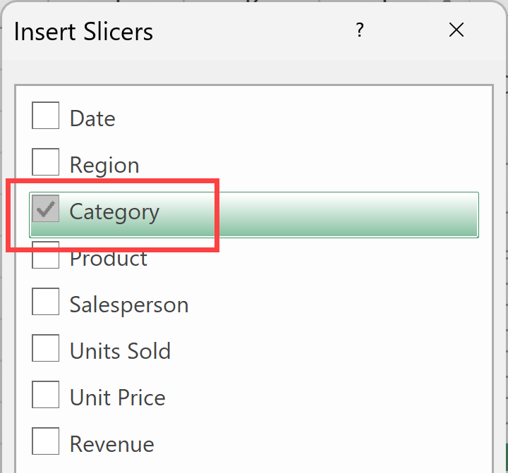
5. Click OK

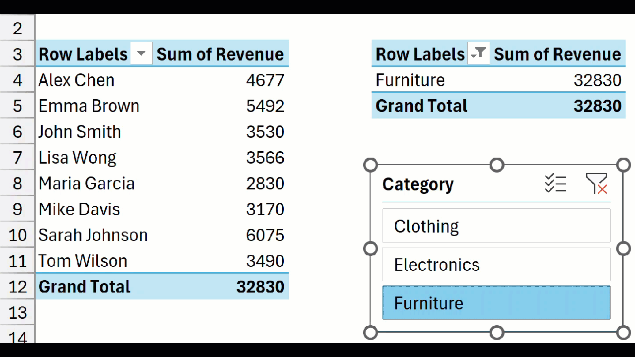
The above steps would insert a slicer in your sheet as shown below.

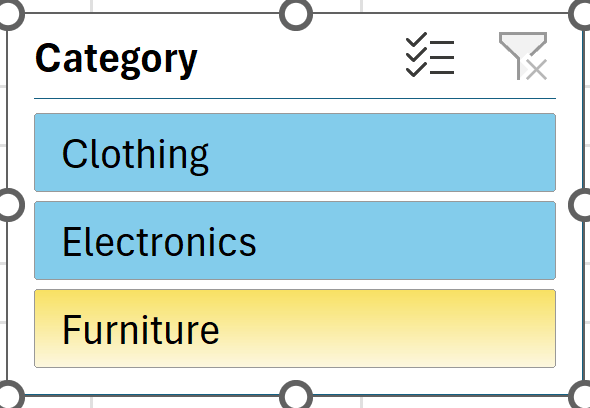
At this point, you’ll notice that the slicer only controls the first pivot table. So if I select the Clothing option in the slicer, it would only update the first Pivot table and not the second one.

So let’s connect the second Pivot table to the same slicer.

1. Right-click on the slicer
2. Click on Report Connections

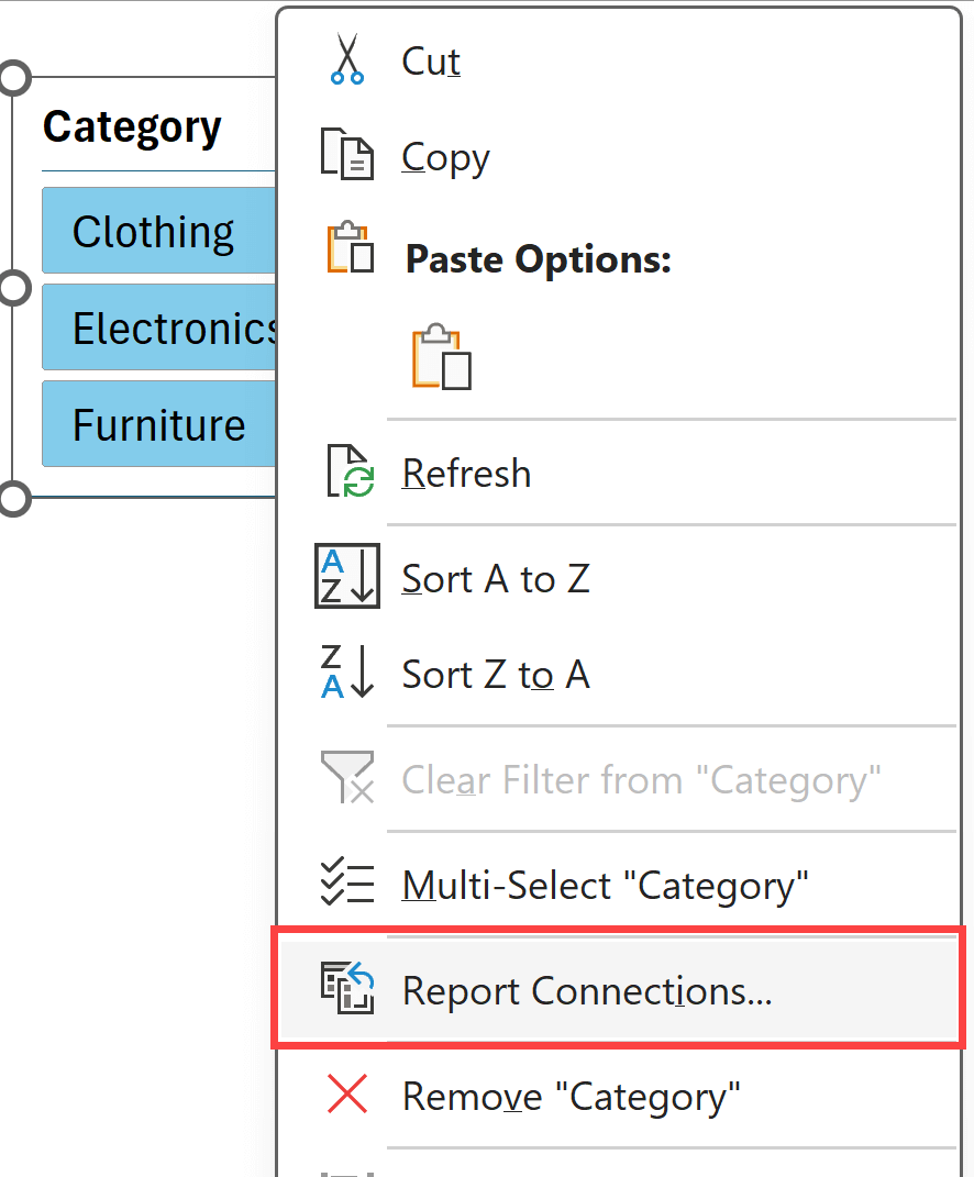
3. In the dialog box that appears, you’ll see both Pivot Tables listed (this confirms they share the same data source)
4. Check the box next to the second pivot table

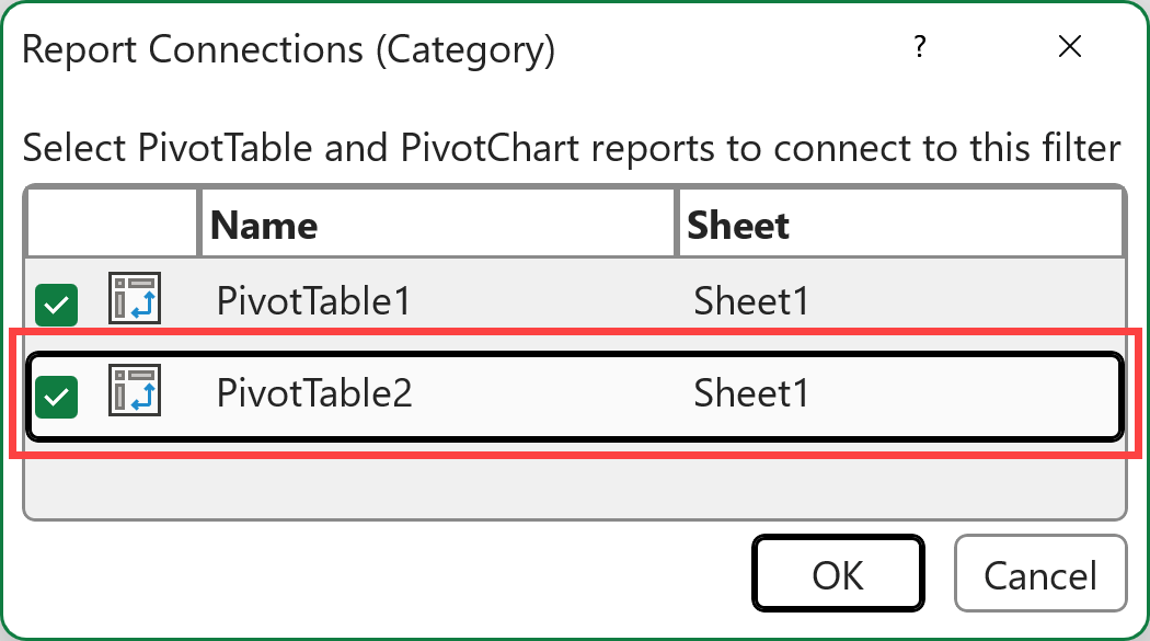
5. Click OK

And we’ve done it!

Now when you make selections in your slicer, both pivot tables will update simultaneously.

Pro Tip: To select multiple items in a slicer, hold the Ctrl key while clicking on different options.

Scenario 2: Connecting Slicer to Pivot Tables Created from Different Data Sources

This scenario is more complex (and more common).

Sometimes you have related data stored in separate tables that you want to analyze together.

For this to work, there needs to be a common field between the datasets that can serve as a connecting point.

Data Sources

Let’s say I have two different data sources that are used to create two different pivot tables that I want to control with one single slicer.

• Data 1: Sales transaction records with columns like Date, Region, Category, Salesperson, and Revenue

• Data 2: Salesperson details with columns like Salesperson, Reporting Manager, Hire Date, Experience, and Base Salary

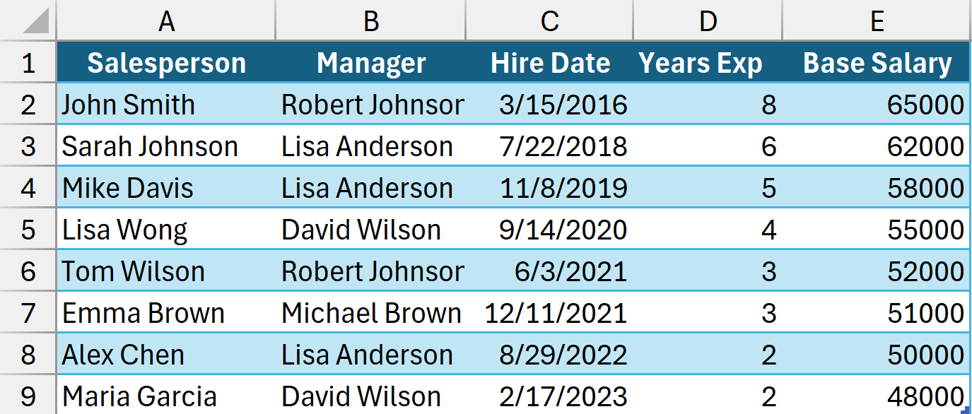
The common field here is “Salesperson,” which appears in both datasets (and each Salesperson’s name only appears once in the Data 2 table).

Important Requirements

For this technique to work:

• There must be at least one common field between your datasets
• In the lookup table (Data 2), the common field values should be unique (no duplicates)
• The common field values should match exactly between both datasets

Step 1 – Creating Pivot Tables with Data Model

In this step, we are going to create two pivot tables using two separate data sources and add these pivot tables to a data model.

This will allow us to create a relationship between these two data sources.

Creating the First Pivot Table:

1. Select any cell in your first dataset
2. Go to Insert tab and then click on PivotTable. This will open the PivotTable from table or range dialog box

3. Choose New Worksheet

4. **Important** Check the box that says “Add this data to the Data Model“

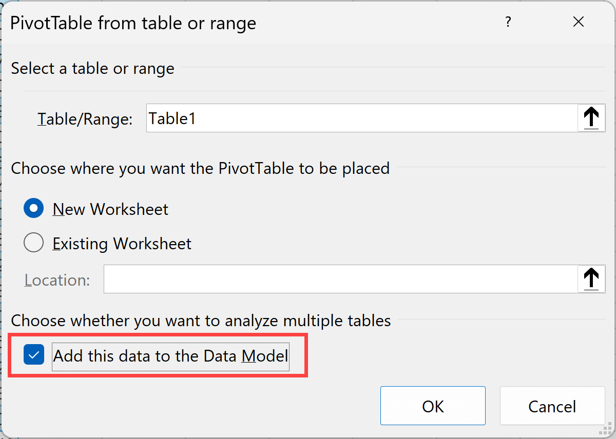
5. Click OK

For now, let’s leave the Pivot Table blank as we can configure it later once we have created the relationship between the two data sources.

Creating the Second Pivot Table:

1. Select any cell in your second dataset
2. Go to Insert tab and then click on PivotTable. This will open the PivotTable from table or range dialog box
3. Again, check “Add this data to the Data Model“
4. Choose Existing Worksheet and select where you want it (alternatively, you can also choose to have this in a new worksheet).
5. Click OK

For now, let’s leave the Pivot Table blank as we can configure it later once we have created the relationship between the two data sources.

Step 2 – Creating Relationships in Power Pivot

Now, this is the step where magic happens.

Since we added both of these data sources in the data model while creating the Pivot table, we will now be able to create a relationship between these two data sources using Power Pivot.

Here are the steps to do this:

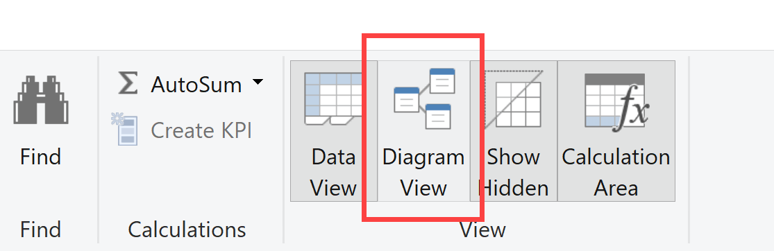
1. Go to the Power Pivot tab in the ribbon
2. Click on the Manage icon

3. In the Power Pivot window, click on Diagram View. You’ll see both tables displayed here

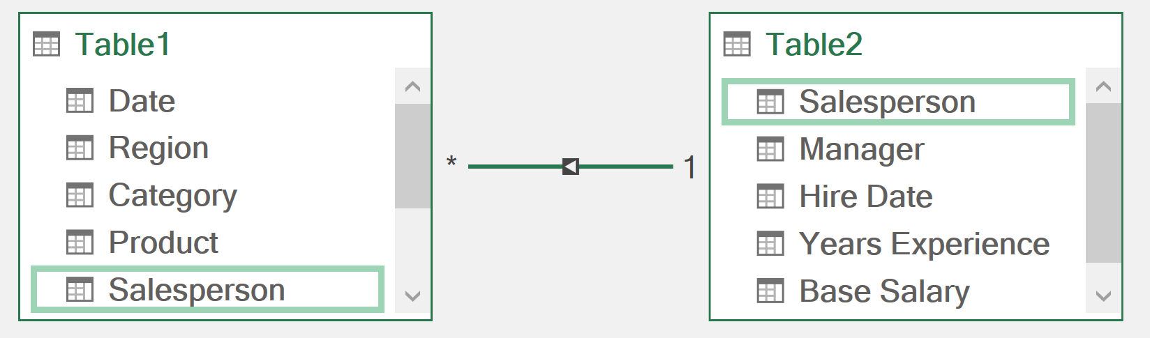
4. Drag the common field from one table to the corresponding field in the other table. In this example, since the common link is the Salesperson name, I will drag the Salesperson field from one table to another, which is going to create a relationship (you’ll see a line connecting the tables).

5. Close the Power Pivot window

Note: The relationship will be “one-to-many” where one table has unique values (like employee details) and the other has multiple transactions per person.

Step 3 – Configuring the Pivot Tables

We did not configure the pivot tables to show us the results because I first wanted to create the relationship in the Power Pivot.

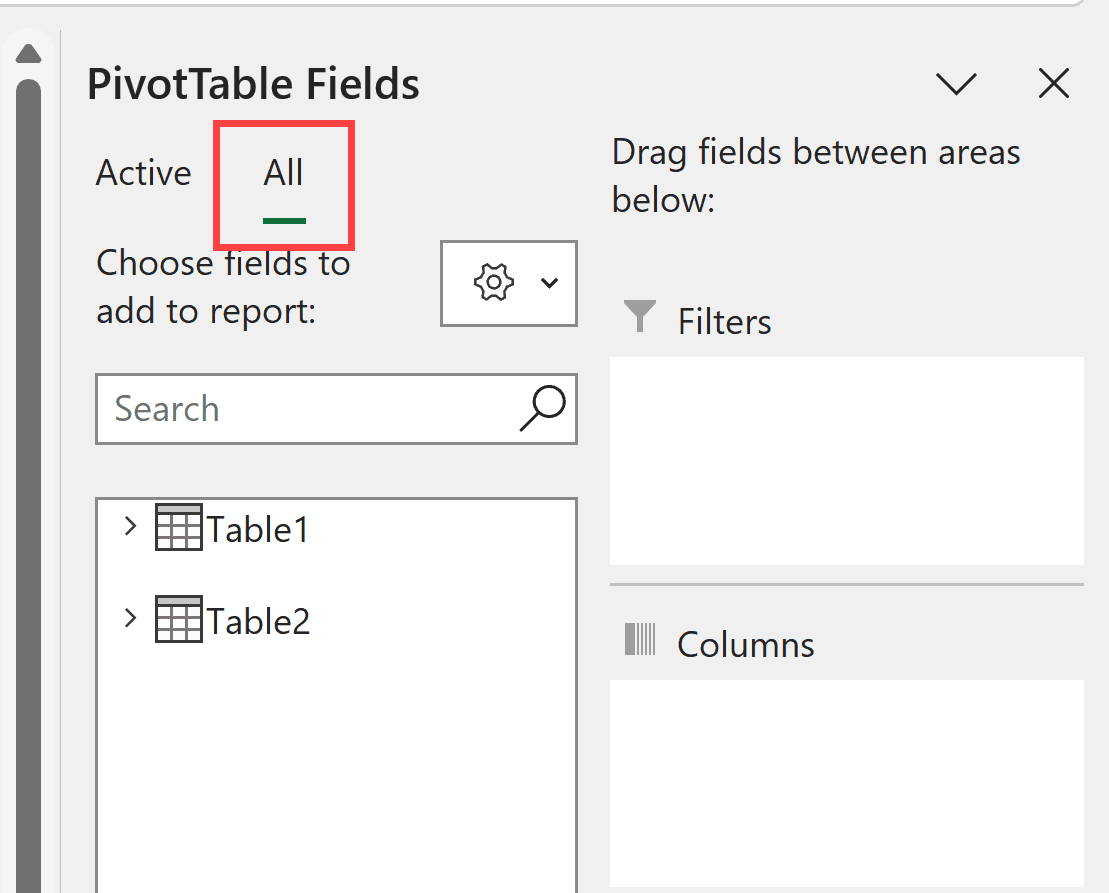
Once you create a relationship in Power Pivot, you’ll notice that fields from both pivot tables are now available for use in each pivot table.

So if you select a cell in any of the Pivot Tables and then look at the PivotTable Fields pane, you’ll notice that it has a new tab called ‘All’. When you click on it, it will show you all the tables that are connected and can be used for this pivot table.

So now let’s configure both of these Pivot tables.

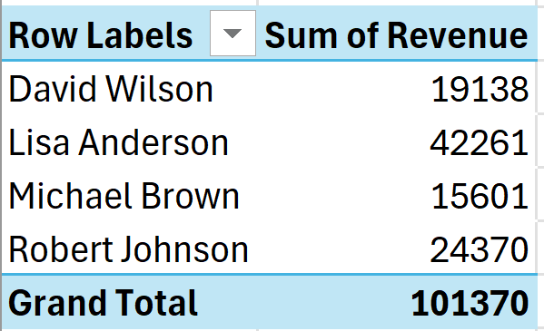
For the first Pivot table, I will put Salesperson in the rows area and the Revenue in the Values area. This will give me a pivot table as shown below.

For the second Pivot table, I will put Manager in the rows area and the Revenue in the Values area. Interestingly, note that the Manager field is from a different data source, and the Revenue field is from a different data source.

The reason I am able to create a Pivot table using fields from two different data sources is because I have created a relationship between them. This allows me to treat these Pivot tables as one combined data source.

This will give me a Pivot table as shown below.

Step 4 – Connecting the Slicer

Now that we have two Pivot tables that use two different data sources that have been connected using Power Pivot, let’s create a slicer that can control both of these Pivot tables.

Here are the steps to do this:

1. Select any cell in the first Pivot table we created
2. Go to PivotTable Analyze tab and then click on the Insert Slicer option

4. Choose your desired field (let’s use Category in this example)

5. Click OK. This will insert the slicer in the worksheet.
6. Right-click on the slicer and select Report Connections. You will see both Pivot table names listed here, and this is possible because we created a connection in Power Pivot.

7. Check the box for the second pivot table

5. Click OK

Voila!

Now both Pivot tables will respond to the same slicer, even though they were created from different data sources!

Few Things to Keep in Mind

• Pivot tables can expand and contract based on data, so it’s generally better to place them on separate worksheets
• Large datasets with multiple relationships can slow down your workbook
• For different data sources, ensure your common fields have exact matches (watch out for extra spaces, different capitalizations, etc.)
• Clean your data before creating relationships to avoid connection issues

Troubleshooting Common Issues

Slicer doesn’t affect the second pivot table: Make sure both pivot tables are properly connected through Report Connections.

Can’t see both pivot tables in Report Connections: This usually means the pivot tables don’t share a common data source or haven’t been properly added to the Data Model.

Relationship creation fails: Check that your common fields have matching data types and that the lookup table doesn’t have duplicate values in the key field.

I hope you found this article helpful.

If you have any questions or suggestions for me, please let me know in the comments area.

Other Excel articles you may also like:

• How to Refresh Pivot Table in Excel
• Preparing the Source Data For Pivot Table
• How to Apply Conditional Formatting in a Pivot Table in Excel
• How to Show Pivot Table Fields List? (Get Pivot Table Menu Back)
• How to Filter Data in a Pivot Table in Excel