Fill Down Blank Cells Until the Next Value in Excel (3 Easy Ways)

Watch Video – Fill Down in Excel

A lot of times, you may encounter a data set where only one cell is filled with data and the cells below it are blank till the next value.

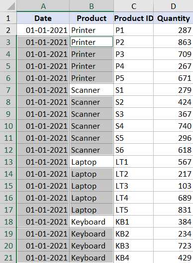
Something as shown below:

While this format works for some people, the problem with this sort of data is that you cannot use it to create Pivot Tables or use it in calculations.

And this has an easy fix!

In this tutorial, I will show you how to quickly fill down cells in Excel until the next filled value.

You can easily do this using a simple Go-To special dialog box technique, VBA, or Power Query.

So let’s get started!

Method 1 – Fill Down Using Go To Special + Formula

Suppose you have a data set as shown below and you want to fill down data in column A and column B.

In column B, the aim is to fill ‘Printer’ till the last empty cell below it, and then when ‘Scanner’ starts, then fill ‘Scanner’ in the cells below till the cells are empty.

Below the steps to use go to special to select all the blank cells and fill down using a simple formula:

1. Select the data in which you want to fill down (A1:D21 in our example)
2. Go to the ‘Home’ tab

3. In the Editing group, click on the ‘Find & Select’ icon (this will show some more options in the drop-down)

4. Click on the ‘Go To’ option

5. In the Go-To dialog box that opens up, click on the Special button. This will open the ‘Go To Special’ dialog box

6. In the Go To Special dialog box, click on Blanks

7. Click OK

The above steps would select all the blank cells in the data set (as shown below).

In the blank cells that are selected, you would notice that one cell is lighter than the rest of the selection. This cell is the active cell where we’re going to enter a formula.

Don’t worry about where the cell is in the selection, as our method would work in any case.

Now, below are the steps to fill down the data in the selected blank cells:

1. Hit the equal-to (=) key on your keyboard. This will insert an equal to sign in the active cell
2. Press the up arrow key. This will insert the cell reference of the cell above the active cell. For example, in our case, B3 is the active cell and when we do these two steps, it enters =B2 in the cell
3. Hold the Control key, and press the Enter key

The above steps would automatically insert all the blank cells with the value above them.

While this may look like too many steps, once you get the hang of this method, you’ll be able to quickly fill-down data in Excel within a few seconds.

Now, there are two more things that you need to take care of when using this method.

Convert Formulas to Values

The first one is to make sure that you convert formulas to values (so that you have static values and things don’t mess up in case you change data in the future).

Below is a video that will show you how to quickly convert formulas to values in Excel.

Change the Date Format

In case you’re using dates in your data (as I am in the example data), you would notice that the filled-down values in the date column are numbers and not dates.

If the output in the date column are in the desired date format, you’re good and don’t need to do anything else.

But if these are not in the correct date format, you need to make a minor adjustment. While you have the right values, you just need to change the format so that it is displayed as a date in the cell.

Below are the steps to do this:

1. Select the column that has the dates
2. Click the Home tab
3. In the Number group, click on the Format drop-down and then select the date format.

If you need to do this fill-down once in a while, I recommend you use this Go-To special and formula technique.

Although it has a few steps, it’s simple and gives you the result right there in your dataset.

But in case you have to do this quite often, then I suggest you look at the VBA and the Power Query methods covered next

Method 2 – Fill Down Using a Simple VBA Code

You can use a really simple VBA macro code to quickly fill down cells in Excel till the last empty value.

You only need to add the VBA code to the file once and then you can easily reuse the code multiple times in the same workbook or even multiple workbooks on your system.

Below is the VBA code that will go through each cell in the selection and fill down all the cells that are blank:

'This VBA code is created by Sumit Bansal from TrumpExcel.com
Sub FillDown()
For Each cell In Selection
  If cell = "" Then
    cell.FillDown
  End If
Next
End Sub

The above code uses a For loop to go through each cell in the selection.

Within the For loop, I have used an If-Then condition that checks whether the cell is empty or not.

In case the cell is empty, it is filled with the value from the cell above, and in case it is not empty, then the for loop simply ignores the cell and moves to the next one.

Now that you have the VBA code, let me show you where to put this code in Excel:

1. Select the data where you want to fill down
2. Click the Developer tab

3. Click on the Visual Basic icon (or you can use the keyboard shortcut ALT + F11). This will open the Visual Basic Editor in Excel

4. In the Visual Basic Editor, on the left, you would have the Project Explorer. If you don’t see it, click on the ‘View’ option in the menu and then click on Project Explorer

5. In case you have multiple Excel workbooks open, Project Explorer would show you all the workbook names. Locate the workbook name where you have the data.
6. Right-click on any of the objects in the workbook, go to Insert, and then click on Module. This will insert a new module for that workbook

7. Double-click on the ‘Module’ you just inserted in the above step. It will open the code window for that module

8. Copy-paste the VBA code into the code window

9. Place the cursor anywhere in the code and then run the macro code by clicking on the green button in the toolbar or using the keyboard shortcut F5

The above steps would run the VBA code and your data would be filled down.

If you want to use this VBA code again in the future, you need to save this file as a macro-enabled Excel workbook (with a .XLSM extension)

Another thing you can do is add this macro to your Quick Access Toolbar, which is always visible and you’ll have access to this macro with a single click (in the workbook where you have the code in the backend).

So, the next time you have data where you need to fill-down, all you need to do is make the selection and then click on the macro button in the Quick Access Toolbar.

You can also add this macro to the Personal Macro Workbook and then use it in any workbook on your system.

Click here to read more about personal macro workbooks and how to add code to them.

Method 3 – Fill Down Using Power Query

Power Query has an inbuilt functionality that allows you to fill-down with a single click.

Using Power Query is recommended when you’re using it anyway to transform your data or combine data from multiple worksheets or multiple workbooks.

As a part of your existing workflow, you can use the fill-down option in Power Query to quickly fill the blank cells.

To use Power Query, it’s recommended that your data is in an Excel Table format. If you can’t convert your data into an Excel table, you will have to create a named range for the data and then use that named range in Power Query.

Below I have the data set that I have converted into an Excel table already. You can do that by selecting the dataset, going to the Insert tab, and then clicking on the Table icon.

Below the steps to use Power Query to fill down data till the next value:

1. Select any cell in the data set
2. Click the Data tab

3. In the Get & Transform Data group, click on ‘From Sheet’. This will open the Power Query editor. Note that the blank cells would show the value ‘null’ in Power Query

4. In the Power Query editor, select the columns for which you want to fill down. To do this, hold the Control key and then click on the header of the columns that you want to select. In our example, it would be the Date and the Product columns.
5. Right-click on any of the selected headers

6. Go to the ‘Fill’ option and then click on ‘Down’. This would fill down the data in all the blank cells

7. Click the File tab and then click on ‘Close & Load’. This will insert a new worksheet in the workbook with the resulting table

While this method may sound a bit of an overkill, one great benefit of using Power Query is that it allows you to quickly update the resulting data in case your original data changes.

For example, if you add more records to the original data, you don’t need to do all the above again. You can simply right-click on the resulting table and then click on Refresh.

While the Power Query method works well, it’s best to use it when you’re already using Power Query in your workflow.

If you just have a dataset where you want to fill down the blank cells, then using the Go To special method or the VBA method (covered above) would be more convenient.

So these are three simple ways that you can use to fill down blank cells until the next value in Excel.

I hope you found this tutorial useful.

Other Excel tutorials you may also like:

• How to use Fill Handle in Excel
• How to Quickly Fill Numbers in Cells without Dragging
• 10 Excel Data Entry Tips You Can’t Afford to Miss
• How to Highlight Blank Cells in Excel
• How to Use Flash Fill in Excel
• How to Edit Cells in Excel?