
With Power Query, working with data dispersed across worksheets or even workbooks has become easier.
One of the things where Power Query can save you a lot of time is when you have to merge tables with different sizes and columns based on a matching column.
Below is a video where I show exactly how to merge tables in Excel using Power Query.
In case you prefer reading the text over watching a video, below are the written instructions.
Suppose you have a table as shown below:
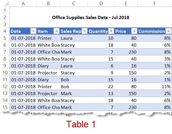
This table has the data I want to use, but it’s still missing two important columns – the ‘Product Id’ and the ‘Region’ where the sales rep operates.
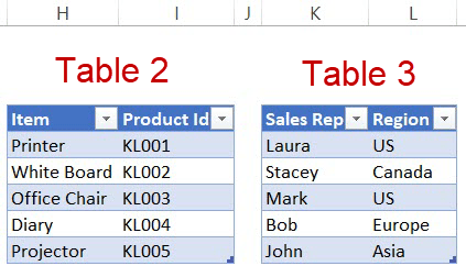
This information is provided as separate tables as shown below:
To get all this information into a single table, you will have to merge these three tables so that you can then create a Pivot Table and analyze it, or use it for other reporting/dashboarding purposes.
And by merging, I don’t mean a simple copy paste.
You’ll have to map the relevant records from Table 1 with data from Table 2 and 3.
Now you can rely on VLOOKUP or INDEX/MATCH to do this.
Or if you’re a VBA whiz, you can write a code to do this.
But these options are time-consuming and complicated as compared with Power Query.
In this tutorial, I will show you how to merge these three Excel tables into one.
For this technique to work, you need to have connecting columns. For example, in Table 1 and Table 2, the common column is ‘Item’, and in Table 1 and Table 3, the common column is ‘Sales Rep’. Also, note that there should be no repetition in these connecting columns.
Note: Power Query can be used as an add-in in Excel 2010 and 2013, and is an inbuilt feature from Excel 2016 onwards. Based on your version, some images may look different (image captures used in this tutorial are from Excel 2016).
Merge Tables Using Power Query
I have named these tables as shown below:
- Tabel 1 – Sales_Data
- Table 2 – Pdt_Id
- Table 3 – Region
It isn’t mandatory to rename these tables, but it’s better to give names that describe what the table is about.
At one go, you can merge only two tables in Power Query.
So we will first have to merge Table 1 and Table 2 and then merge Table 3 into it in the next step.
Merging Table 1 and Table 2
To merge tables, you first need to convert these tables into connections in Power Query. Once you have the connections, you can easily merge these.
Here are the steps to save an Excel table as a connection in Power Query:
- Select any cell in Sales_Data table.
- Click the Data tab.

- In the Get & Transform group, click on ‘From Table/Range’. This will open the Query editor.

- In the Query editor, click the ‘File’ tab.

- Click on ‘Close and Load To’ option.

- In the ‘Import Data’ dialog box, select ‘Only Create Connection’.

- Click OK.
The above steps would create a connection with the name Sales_Data (or any name that you have given to the Excel Table).
Repeat the above steps for Table 2 and Table 3.
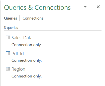
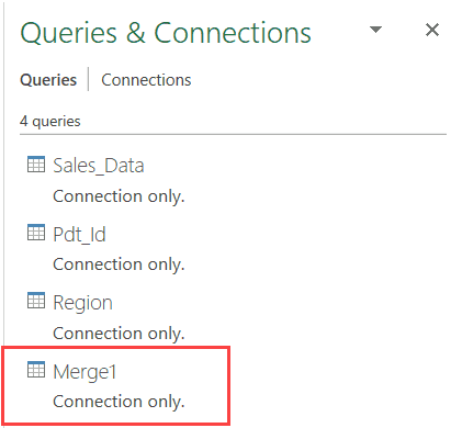
So when you’re done, you will have three connections (with the name Sales_Data, Pdt_Id, and Region).
Now let’s see how to merge the Sales_Data and Pdt_Id table.
- Click on the Data tab.
- In the Get & Transform Data group, click on Get Data.

- In the drop-down, click on Combine Queries.
- Click on Merge. This will open the Merge dialog box.

- In the Merge dialog box, select ‘Sales_Data’ from the first drop down.

- Select ‘Pdt_Id’ from the second drop down.

- In ‘Sales_Data’ preview, click on the ‘Item’ column. Doing this will select the entire column.
- In ‘Pdt_Id’ preview, click on the ‘Item’ column. Doing this will select the entire column.
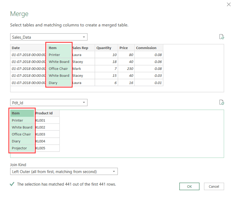
- In the ‘Join Kind’ drop-down, select ‘Left Outer (all from first, matching from second)’.

- Click OK.
The above steps would open the Query editor and show you the data from the Sales_Data with one additional column (of Pdt_Id).
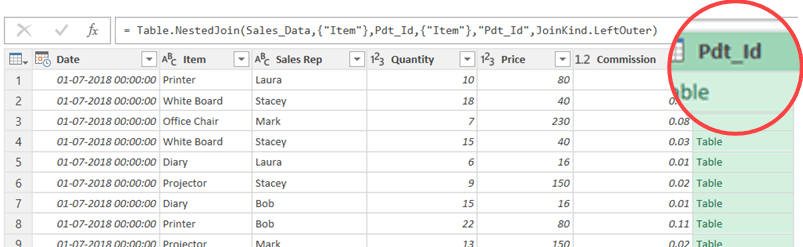
Merging the Excel Tables (Table 1 & 2)
Now the process of merging the tables will happen within the Query editor with the following steps:
- In the additional column (Pdt_Id), click on the double pointed arrow in the header.
- From the options box that opens, uncheck all the column names and only select Item. This is because we already have the product name column in the existing table, and we only want the product ID for each product.
- Uncheck the option ‘Use original column name as prefix’.
- Click Ok.
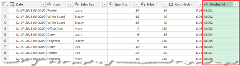
This would give you the resulting table that has every record from Sales_Data table and an additional column that has product ids as well (from the Pdt_Id table).
Now if you only want to combine two tables, you can load this Excel you’re done.
But we have three tables to merge, so there is more work to be done.
You need to save this resulting table as a connection (so that we can use it to merge it with Table 3).
Here are the steps to save this merged table (with data from Sales_Data and Pdt_Id table) as a connection:
- Click the File tab
- Click on ‘Close and Load to’ option.
- In the ‘Import Data’ dialog box, select ‘Only Create Connection’.
- Click OK.
This will save the newly merged data as a connection. You can rename this connection if you want.
Merging Table 3 with the Resulting Table
The process of merging the third table with the resultant table (that we got by merging Table 1 and Table 2) is exactly the same.
Here are the steps to merge these tables:
- Click on the Data tab.
- In the Get & Transform Data group, click on ‘Get Data’.
- In the drop-down, click on ‘Combine Queries.
- Click on ‘Merge’. This will open the Merge dialog box.
- In the Merge dialog box, Select ‘Merge1’ from the first drop down.
- Select ‘Region’ from the second drop down.
- In ‘Merge1’ preview, click on the ‘Sales Rep’ column. Doing this will select the entire column.
- In Region preview, click on the ‘Sales Rep’ column. Doing this will select the entire column.
- In the ‘Join Kind’ drop-down, select Left Outer (all from first, matching from second).
- Click OK.
The above steps would open the Query editor and show you the data from Merge1 with one additional column (Region).
Now the process of merging the tables will happen within the Query editor with the following steps:
- In the additional column (Region), click on the double pointed arrow in the header.
- From the options box that opens, uncheck all the column names and only select Region.
- Uncheck the option ‘Use original column name as prefix’.
- Click Ok.
The above steps would give you a table that has all the three tables merged (Sales_Data table with one column for Pdt_Id and one for Region).
Here are the steps to load this table in Excel:
- Click the File tab.
- Click on ‘Close and Load to’.
- In the ‘Import Data’ dialog box, select Table and New Worksheets options.
- Click OK.
This would give you the resulting merged table in a new worksheet.
One of the best things about Power Query is that you can easily accommodate any changes in the underlying data (Table 1, 2 and 3) by simply refreshing it.
For example, suppose Laura gets transferred to Asia and you get new data for the next month. Now you don’t have to repeat the above steps again. All you need to do is refresh the table and it will do everything it all over again for you.
Within seconds you’ll have the new merged table.
You May Also Like the Following Power Query Tutorials:
- Combine Data from Multiple Workbooks in Excel (using Power Query).
- Combine Data From Multiple Worksheets into a Single Worksheet in Excel.
- How To Copy Excel Table Into Word
- How to Unpivot Data in Excel using Power Query (aka Get & Transform)
- Get a List of File Names from Folders & Sub-folders (using Power Query)
- Combine CSV Files With Inconsistent Column Headers


This has been super helpful. Thanks bunches
Nice, detailed instructions, but I need to merge data from three tables into one, not create a table with matched entries. i.e. three tables with identical column headers which I need to merge into one table dynamically without having to cut/paste the three into one every time I modify one. Is there a way to do that?
There is a way to do that. Instead of Merge, you should use Append (step 4).
This functionality does not exist in Excel 2013. MISLEADING
Very useful and neat!
شكرا جزيلا
This was very helpful!! Thank you!!
Hi! I am trying to merge tables from a web source that the number of tables varies from day to day. When i import the data connection and use the append in power query, i get the following:
= Table.Combine({#”Table 0″, #”Table 1″, #”Table 10″, #”Table 11″, #”Table 12″, #”Table 13″, #”Table 2″, #”Table 3″, #”Table 4″, #”Table 5″, #”Table 6″, #”Table 7″, #”Table 8″, #”Table 9″})
is there a way to make this dynamic so that it looks for *any* table instead of this static list of tables? Sometimes i have 4 tables, sometimes i have 20… the file name it is reading from is the same but the table count is variable depending on the data… how can i do this?
Thank you for this video, but I can’t get the merge to work, because after creating the connection, in Merge dialog, there is NO Join Kind dropdown. Any suggestions why that might be? Thank you.
Muchas gracias, no tenía ni idea que Excel tuviera esta herramienta.
This is exactly what I needed. Thank you so much!!
amazing ! thank you very much for your valuable contents and learning
Wonderful tutorial! Please can you give the link to the data you used for both write-ups and youtube?