How to Unhide Rows in Excel (3 Easy Ways + Shortcut)

If you have a few rows hidden in your worksheet and you want them back, Excel makes it quick. Most of the time it takes a couple of clicks.

But sometimes you click around, try the obvious things, and the rows still won’t show up. That usually means something else is going on, like an active filter or a row whose height was dragged down to zero.

In this tutorial, I’ll show you three easy ways to unhide rows in Excel, plus the keyboard shortcut I reach for the most. I’ll also cover how to fix the cases where rows refuse to come back.

Method 1: Right-Click and Unhide Rows

This is the simplest way to unhide rows in Excel, and it works whether you have one hidden row or a whole range of hidden rows in between.

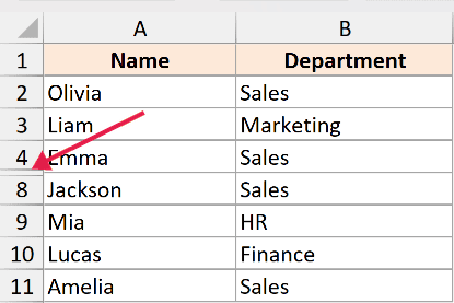
Below, I have a small dataset of 10 employees and their departments, where rows 5 to 7 are hidden. You can tell because the row numbers jump straight from 4 to 8.

Here are the steps to unhide these rows using right-click:

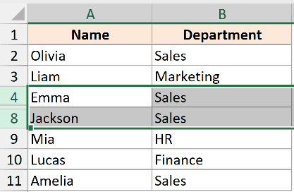
1. Select the rows above and below the hidden ones. In this example, click row number 4, hold Shift, and click row number 8.

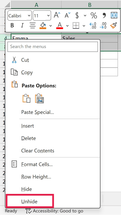
2. Right-click anywhere on the selected row numbers, then click Unhide from the menu.

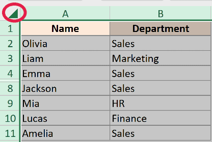
The hidden rows show up right away.

This works the same way whether you’re unhiding one row or fifty. As long as the hidden rows sit between two visible rows you’ve selected, Excel knows what to bring back.

The same approach also works when you need to unhide columns in your worksheet.

Method 2: Unhide All Rows Using the Format Option

This is the method I use when I don’t know exactly where the hidden rows are, or when I want to unhide all the rows in a sheet at once.

It’s also handy when someone hands you a sheet and you suspect there are hidden rows somewhere, but you don’t want to hunt for them.

Here are the steps to unhide all rows using the Format option:

1. Select the entire sheet. Click the small triangle in the top-left corner (between column A and row 1), or press Ctrl + A.

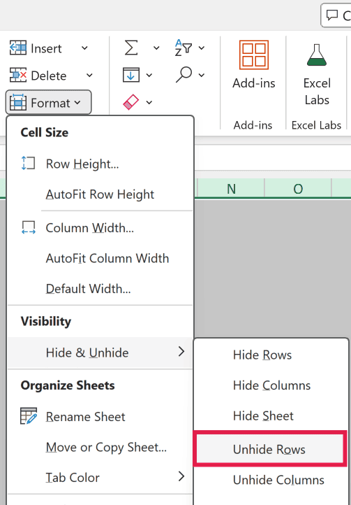
2. On the Home tab, in the Cells group, click Format, then Hide & Unhide, then Unhide Rows.

Every hidden row in the worksheet comes back in one click. This is the safest method when you’re not sure how many rows are hidden or where they are.

Method 3: Double-Click the Row Border

If you’d rather stick with the mouse, you can unhide rows straight from the row numbers on the left.

Here are the steps to unhide a row by double-clicking the border:

1. Hover your cursor right on the line between the two row numbers where the rows are hidden (for example, between row 4 and row 8). The cursor turns into a double-headed arrow.
2. Double-click that line. The hidden rows come back at their normal height.

Instead of double-clicking, you can also click and drag that line downward to set the height yourself.

This is the one method that also rescues a row whose height was dragged down to zero rather than properly hidden.

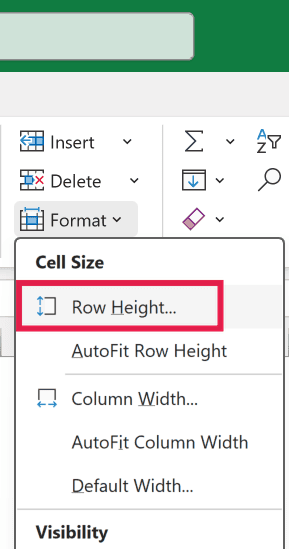
Pro Tip: If dragging feels fiddly, select the row numbers around the hidden one, go to Home > Format > Row Height, type 15, and click OK. That sets the rows back to the default height.

Keyboard Shortcut to Unhide Rows (Ctrl + Shift + 9)

If you want the fastest way to unhide rows in Excel, use the keyboard shortcut Ctrl + Shift + 9.

Here are the steps to use it:

1. Select the rows above and below the hidden ones. Or press Ctrl + A to select the whole sheet if you want to unhide every hidden row.
2. Press Ctrl + Shift + 9.

That’s it. The hidden rows reappear.

Pro Tip: On a Mac, the shortcut is Command + Shift + 9.

This is the shortcut I reach for the most, because it works for a single hidden row and for unhiding multiple rows at the same time. The trick is simply what you select before you press it.

Can’t Unhide Rows in Excel?

This is the part that frustrates people the most. You try every method above and the rows still don’t show up.

Here are the most common reasons, and how to fix each one.

An applied filter is hiding the rows

If a filter is active on your data, the rows that don’t match the filter look hidden, but they’re not. Unhide won’t bring them back because they were never hidden in the first place.

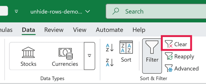
Go to the Data tab and click Clear in the Sort & Filter group. You can also open each column’s filter dropdown and tick Select All.

Frozen panes are hiding the top rows

Sometimes you can’t see row 1, 2, or 3 because frozen panes are scrolled past them.

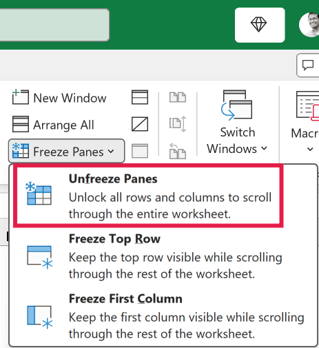
Go to the View tab, click Freeze Panes, and choose Unfreeze Panes. Then scroll back to the top.

The row height is set to 0 instead of being truly hidden

If someone dragged the row border up to 0 rather than using Hide, the regular Unhide command may not reveal it.

Use Method 3 above, or select the rows and go to Home > Format > Row Height and set it to 15.

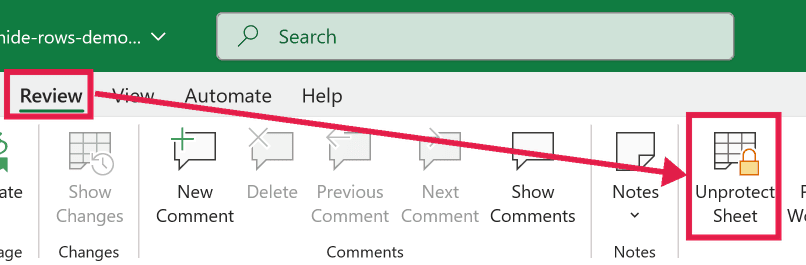
The sheet is protected

If the worksheet is protected, you can’t unhide rows at all. Go to the Review tab and click Unprotect Sheet.

You may need a password if one was set.

Row 1 is hidden and there’s nothing above it to select

When the very first row is hidden, you can’t select the row above it, so right-click won’t offer the Unhide option.

Type A1 in the Name Box (next to the formula bar) and press Enter to land on that hidden cell.

Then go to Home > Format > Row Height, set it to 15, and click OK. The top row comes back.

Things to Keep in Mind

• A truly hidden row and a row with its height set to 0 look the same on screen, but the regular Unhide command works only on truly hidden rows. If Unhide does nothing, set the row height manually.
• A filter is not the same as hidden rows. Filtered rows are tied to your filter criteria, so clear the filter to bring them all back.
• If your data is in an Excel Table, the row numbers keep running normally, but the table may be filtered or sorted in a way that looks like hidden rows. Check the filter arrows on the table headers.
• The Ctrl + Shift + 9 shortcut works for both a single section and the whole sheet. Select the rows around one gap, or press Ctrl + A first to unhide everything at once.
• Protected sheets block every unhide action. If nothing works, the sheet is probably protected, so unprotect it from the Review tab first.
• If your goal is to clean up a workbook full of hidden content, you can delete all hidden rows and columns at once instead of unhiding them. And if entire worksheets are missing, here’s how to unhide sheets in Excel.

That covers the three easy ways to unhide rows in Excel, the Ctrl + Shift + 9 shortcut, and the fixes for when rows just won’t come back.

I hope you found this tutorial helpful.

Other Excel Articles You May Also Like

• How to Insert Multiple Rows in Excel
• How to Delete Rows in Excel (Single or Multiple)?
• How to Change Row Height in Excel