SUBTOTAL Function in Excel

If you have ever used SUM on a filtered list and watched it return the total of the entire dataset instead of just the visible rows, you have run into the exact problem SUBTOTAL was built to solve.

Most people reach for SUM, COUNT, or AVERAGE out of habit, and those functions don’t care about filters at all.

SUBTOTAL does.

It runs the same kinds of calculations, but only on the rows you can currently see.

That sounds like a small thing. It isn’t.

Once you understand how SUBTOTAL handles filtered and hidden rows, you can build filter-aware totals, self-renumbering serial numbers, grand totals that refuse to double-count, and dashboards that switch their own math.

In this article, I’ll start with some basic everyday SUBTOTAL function examples and then work up to a few advanced examples.

SUBTOTAL Function Syntax in Excel

Here is the syntax of the SUBTOTAL function:

=SUBTOTAL(function_num,ref1,[ref2],...)

• function_num is a number that tells SUBTOTAL which calculation to run. 1 to 11 includes manually hidden rows in the result. 101 to 111 ignores them. Both sets always ignore filtered rows.
• ref1, [ref2], … is the range or ranges you want SUBTOTAL to work on.

Here is the full list of function numbers:

Function	function_num (includes hidden rows)	function_num (ignores hidden rows)
AVERAGE	1	101
COUNT	2	102
COUNTA	3	103
MAX	4	104
MIN	5	105
PRODUCT	6	106
STDEV.S	7	107
STDEV.P	8	108
SUM	9	109
VAR	10	110
VAR.P	11	111

Don’t worry about memorizing these. In practice you’ll reach for 9 (sum) and 3 (count) the most, and the 100-series only when you’re hiding rows by hand.

Let’s get into some practical examples of the SUBTOTAL Function in Excel.

Example 1: Sum a Filtered List

Let’s start with the use case that gets SUBTOTAL onto most people’s screens in the first place.

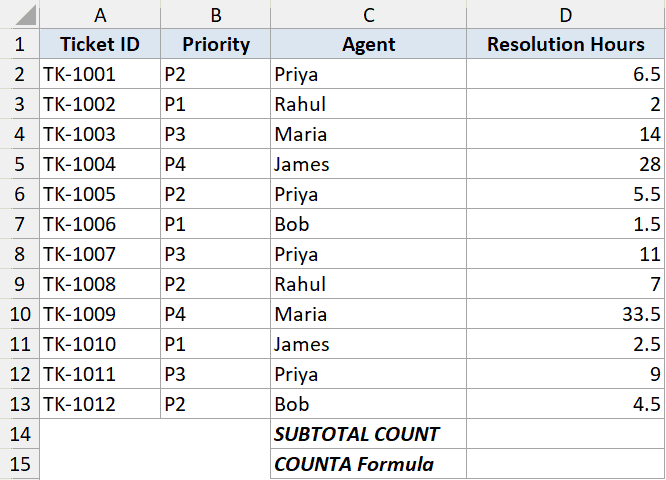
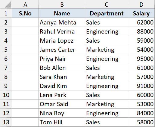
Below is a list of support tickets. Each ticket has an ID, a priority (P1 to P4), the agent who owned it, and the time it took to resolve, in hours.

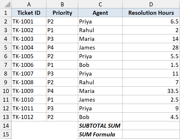
I want a total resolution time that updates whenever I filter the list by priority or by agent. So I’ll put a SUBTOTAL underneath the data, and a plain SUM next to it so we can compare the two.

Here is the SUBTOTAL formula:

=SUBTOTAL(9,D2:D13)

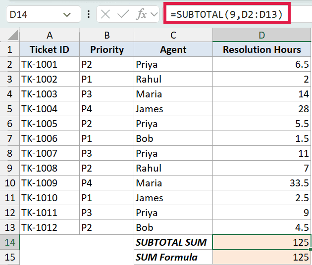
The 9 is the function number for SUM, and with no filter applied this returns 125.

And here is the plain SUM for comparison:

=SUM(D2:D13)

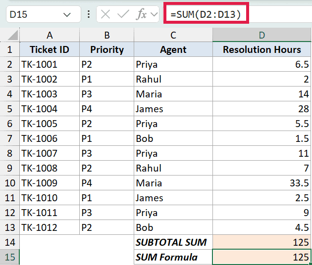
It returns 125 too right now, so the two look identical so far.

Now watch what happens when I filter the list to show only P1 tickets.

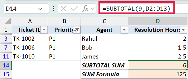
The SUBTOTAL drops to 6, the total of just the visible P1 rows. The plain SUM stays at 125, because it has no idea a filter is even on.

That is the whole point of SUBTOTAL in one screenshot.

Pro Tip: If your data is in an Excel Table, turning on the Total Row (Table Design then Total Row) inserts a SUBTOTAL formula for you automatically. It respects filters out of the box, with a dropdown to switch between sum, count, average, and the rest.

Example 2: Count Visible Rows

This one comes up almost as often as Example 1, and the choice of function number matters.

I’ll use the same support-ticket list. This time I want to know how many tickets are currently visible after I apply a filter, so I’ll compare SUBTOTAL against a plain COUNTA.

Here is the SUBTOTAL formula:

=SUBTOTAL(3,A2:A13)

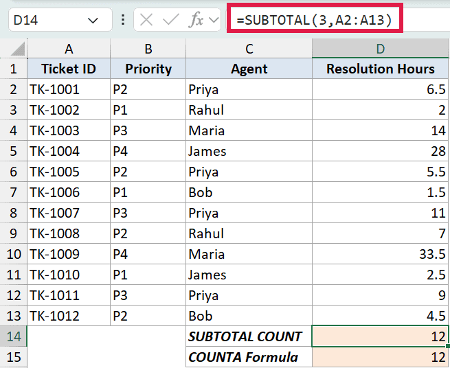
Unfiltered, it counts all 12 visible tickets.

And here is a plain COUNTA on the same column:

=COUNTA(A2:A13)

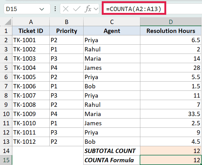
It returns 12 too right now. The difference shows up once you filter.

Filter the list to a single agent and SUBTOTAL falls to the visible count while COUNTA stubbornly stays at 12.

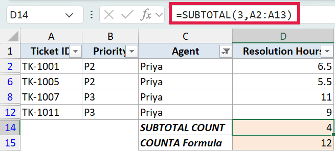
One thing worth knowing here. I used 3 (COUNTA) instead of 2 (COUNT). COUNT only counts numbers. COUNTA counts anything that isn’t blank, including text.

Since ticket IDs are text like TK-1042, 2 would return zero and 3 gives me what I actually want. If you’re counting a numeric column instead, 2 is fine.

Example 3: Function Numbers 9 vs 109 (Manually Hidden Rows)

This is the distinction that trips most people up.

Filters and manually hidden rows are not the same thing. A filter hides rows automatically based on a condition.

A manually hidden row is one you right-clicked and chose Hide on. SUBTOTAL treats them differently, and the function number is how you control that.

Here are my travel expenses, one row per month for the year.

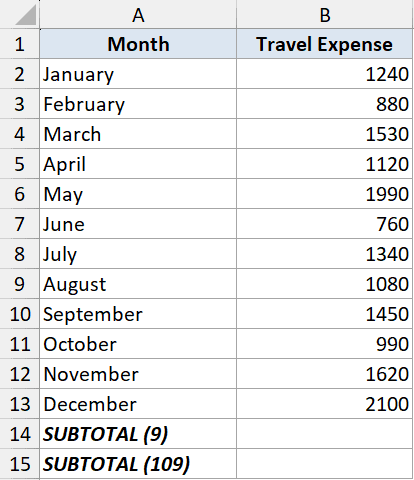
I’ll put two totals underneath. The first uses function number 9:

=SUBTOTAL(9,B2:B13)

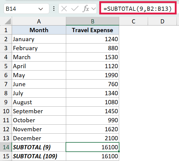
With every row visible, it returns 16,100.

The second uses function number 109:

=SUBTOTAL(109,B2:B13)

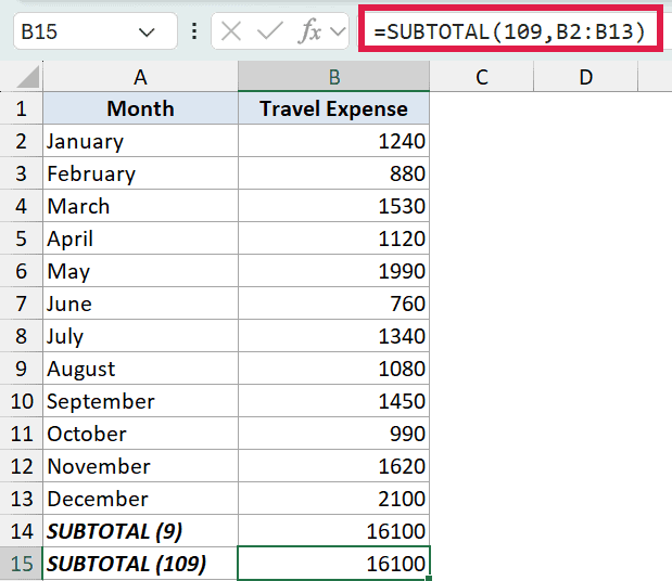
Right now it also returns 16,100. Identical, because nothing is hidden yet.

Now I’ll right-click the May row and choose Hide, the way you might exclude a month from a reimbursement claim.

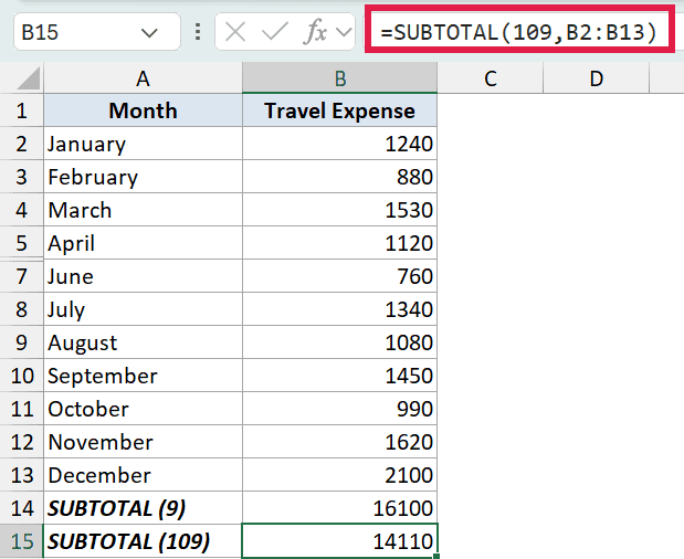
The 9 formula still shows 16,100. It includes May because 9 only respects filters, not manually hidden rows. The 109 formula drops to 14,110 because the 100-series ignores any row you hide by hand, on top of ignoring filtered rows.

A quick recap:

• 1 to 11: ignore filtered rows, but include manually hidden rows
• 101 to 111: ignore filtered rows AND manually hidden rows

If your data only ever uses filters, the two sets behave identically. The distinction only kicks in when someone is hiding rows by hand.

Example 4: Filter-aware Serial Numbers

Here’s a small trick that’s surprisingly useful once you’ve seen it.

Here’s a short employee list. I want a serial-number column on the left that always reads 1, 2, 3 from the first visible row, even after I filter, instead of leaving gaps where rows are hidden.

Here is the formula in the serial-number column, starting from the first data row and filled down:

=SUBTOTAL(3,$B$2:B2)

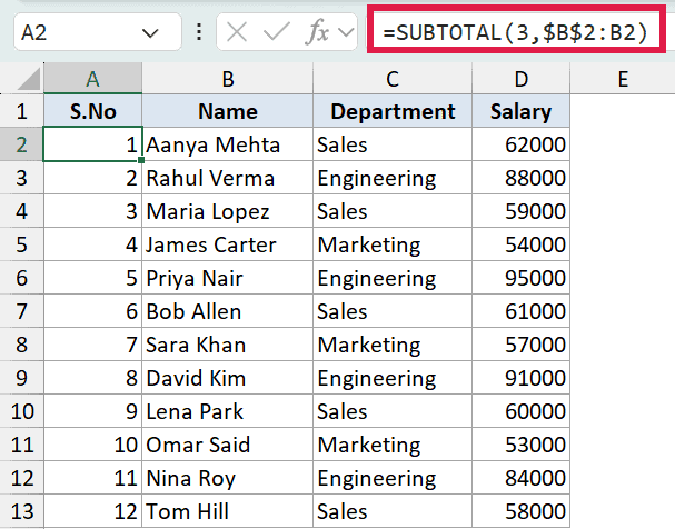
How this formula works:

• The first reference $B$2 is locked. It anchors the range to the first data row.
• The second reference B2 is relative. It grows by one row each time you fill the formula down.
• So row 2 counts B2:B2 and returns 1, row 3 counts B2:B3 and returns 2, and so on.

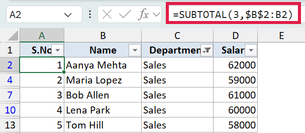
Because SUBTOTAL ignores filtered rows, the count restarts from 1 on whatever row is visible at the top. Filter the list to the Sales department and the numbers shift to match.

This is one of the few times I deliberately fill a formula down each row. The expanding-anchor reference is what makes the trick work, and a single spilling formula wouldn’t give you per-row serial numbers.

Example 5: More Than SUM (Average, Max, and Min on Filtered Data)

People think of SUBTOTAL as a sum tool, but the function number lets it do a lot more. Average, max, min, count, product, even standard deviation, all of them filter-aware.

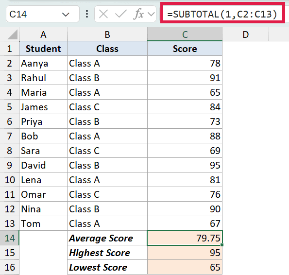
I’ve got a set of student exam scores here, each tagged with a class.

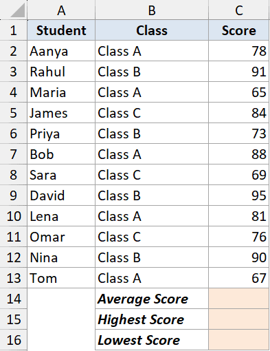
I’ll build a small summary card with three SUBTOTAL formulas. First the average, with function number 1:

=SUBTOTAL(1,C2:C13)

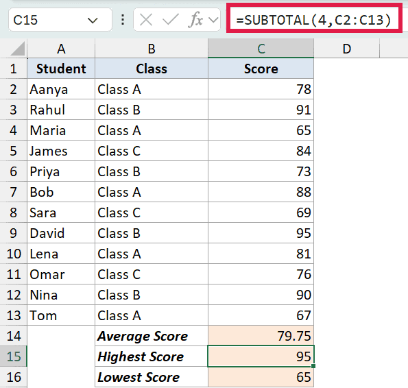
Next the highest score, with function number 4 for MAX:

=SUBTOTAL(4,C2:C13)

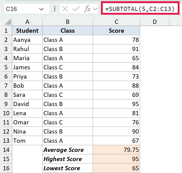
And the lowest score, with function number 5 for MIN:

=SUBTOTAL(5,C2:C13)

Now the payoff. When I filter the list to Class A, all three values recompute on just the visible students. The average, the highest, and the lowest all update together.

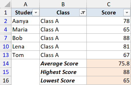
That is a live summary panel for a filtered list, built from three short formulas. No pivot table required.

Example 6: A Grand Total That Ignores Subtotals

This is the cleverest thing SUBTOTAL does, and the least obvious.

SUBTOTAL ignores other SUBTOTAL results inside its own range. That means you can drop a grand total over a list that already has subtotal rows in it, and it won’t double-count.

This next sheet breaks sales out by region, and each region already has its own subtotal row built with SUBTOTAL.

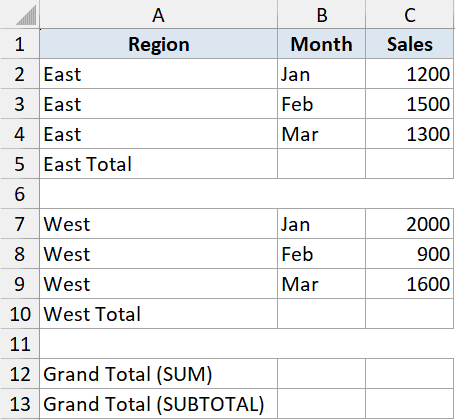
The East subtotal is =SUBTOTAL(9,C2:C4) and the West subtotal is =SUBTOTAL(9,C6:C8). Now I want a grand total across the whole column. Watch what a plain SUM does first:

=SUM(C2:C9)

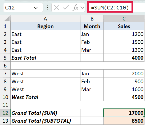
SUM returns 17,000, which is exactly double the real figure. It added the three East values, the three West values, AND the two subtotal rows. The subtotals got counted twice.

Now the same range with SUBTOTAL:

=SUBTOTAL(9,C2:C9)

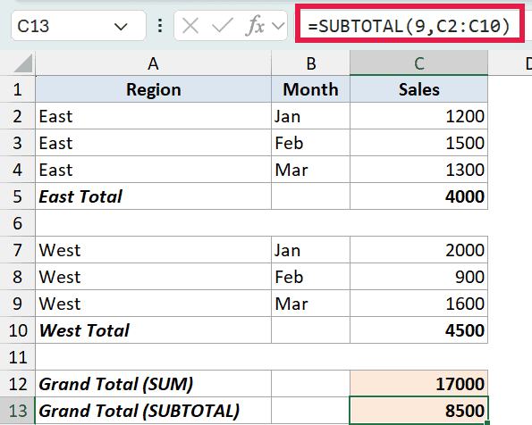
SUBTOTAL returns 8,500, the correct figure.

It skipped the East and West subtotal cells because they are SUBTOTAL formulas themselves. You can stack subtotals and a grand total in one column and nothing gets counted twice.

This same trick is what powers Excel’s built-in Subtotal tool (the one on the Data tab that auto-inserts subtotal rows). Click any row it creates and you’ll see a SUBTOTAL formula in the formula bar. That’s how it can add a grand total at the bottom without double-counting the subtotal rows above it.

Example 7: Conditionally Sum Only the Visible Rows

This one is where SUBTOTAL pulls off something a plain function can’t.

On its own, SUBTOTAL respects filters but takes no conditions. SUMIFS takes conditions but ignores filters. What if you want both, a conditional total that also respects the filter?

You combine SUBTOTAL with SUMPRODUCT and OFFSET. Here’s a list of deals, one per rep, tagged by region.

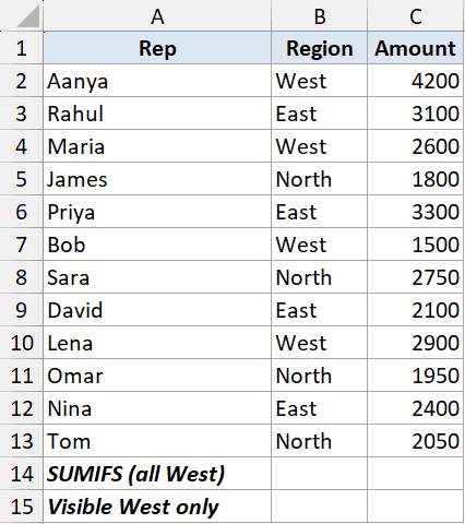
I’ll put two totals for the West region underneath. First a normal SUMIFS:

=SUMIFS(C2:C13,B2:B13,"West")

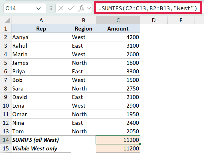
With nothing filtered, it returns 11,200.

And here is the visible-only version that combines SUBTOTAL with SUMPRODUCT and OFFSET:

=SUMPRODUCT((B2:B13="West")*SUBTOTAL(103,OFFSET(B2,ROW(B2:B13)-ROW(B2),0))*C2:C13)

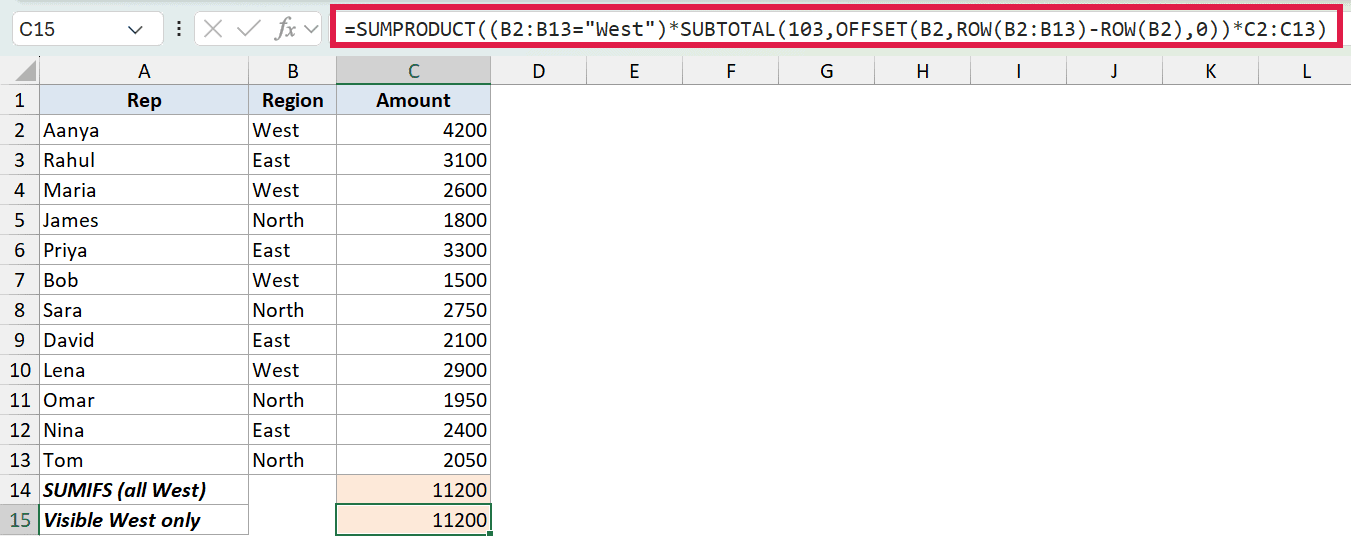
Unfiltered, it also returns 11,200. Now I’ll filter the list to deals over 2,500.

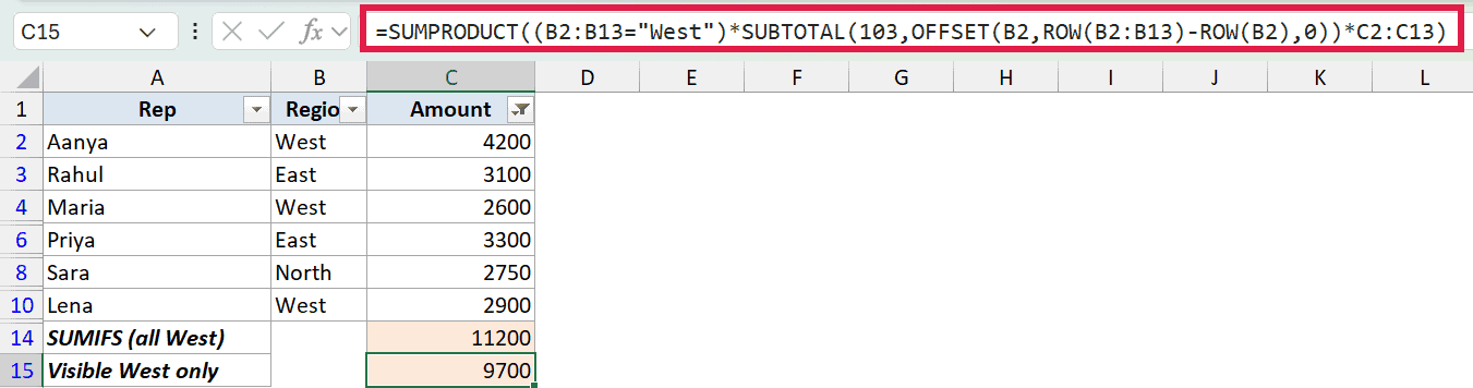
SUMIFS still shows 11,200. It totals every West deal regardless of the filter. The SUBTOTAL version drops to 9,700, the total of just the West deals still visible.

How this formula works:

• OFFSET(B2,ROW(B2:B13)-ROW(B2),0) hands SUBTOTAL one cell at a time down the column.
• SUBTOTAL(103,...) returns 1 for each visible row and 0 for each hidden one.
• (B2:B13="West") returns 1 for West rows and 0 otherwise.
• SUMPRODUCT multiplies the three arrays together, so a row only counts when it is West AND visible, then sums the amounts.

It looks busy, but it is the cleanest way to get a SUMIF that also obeys your filter.

⚠️ One caveat: OFFSET is a volatile function, so this formula recalculates on every change in the workbook. On a list this size you’ll never notice, but on tens of thousands of rows it can slow things down. In that case, add a helper column with =SUBTOTAL(103,B2) filled down (it returns 1 when the row is visible and 0 when it’s hidden) and use a plain =SUMIFS(C2:C13,B2:B13,”West”,D2:D13,1). Same result, no volatility, and you can stack as many conditions as you like.

Example 8: A Dynamic Dashboard with a Dropdown

Because the first argument of SUBTOTAL is just a number, you can make it dynamic. Point it at a cell, drive that cell with a dropdown, and a single formula becomes a mini dashboard.

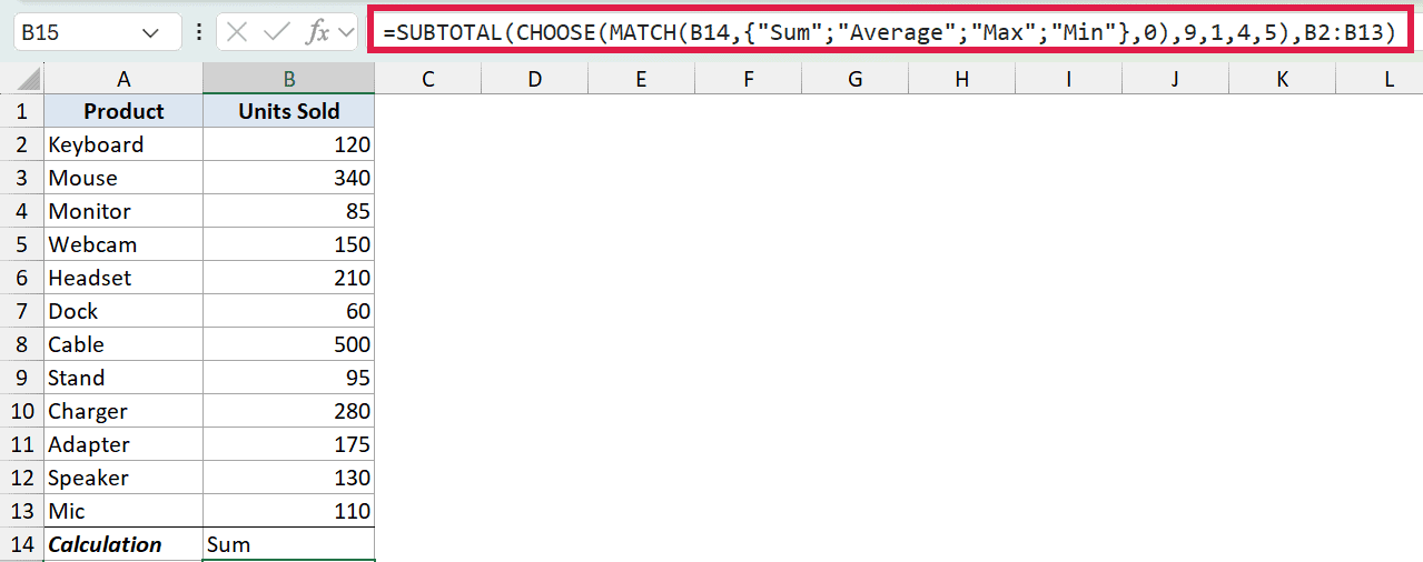
Here’s a list of products and the units sold, with a little control cell underneath.

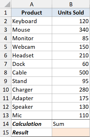
The control cell has a dropdown with Sum, Average, Max, and Min. The result cell uses this formula:

=SUBTOTAL(CHOOSE(MATCH(B14,{"Sum";"Average";"Max";"Min"},0),9,1,4,5),B2:B13)

MATCH finds which word is selected, and CHOOSE turns it into the matching function number (9 for Sum, 1 for Average, 4 for Max, 5 for Min). With the dropdown on Sum, the result is the total units.

Switch the dropdown to Average and the same formula returns the average instead. Nothing else changes.

And because the engine is still SUBTOTAL, the whole thing stays filter-aware. Filter the list to units over 200 and the dashboard total updates to match the visible rows.

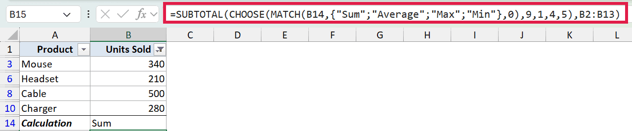
One formula, one dropdown, and you have a summary that switches its own math and respects the filter.

Example 9: SUBTOTAL With a Dynamic Array (FILTER)

One last pattern for Excel 365 users. SUBTOTAL takes references, not arrays, so you can’t drop a FILTER straight inside it. Try =SUBTOTAL(9,FILTER(...)) and Excel rejects the formula. The fix is to let FILTER spill into a helper range first, then point SUBTOTAL at that spill range.

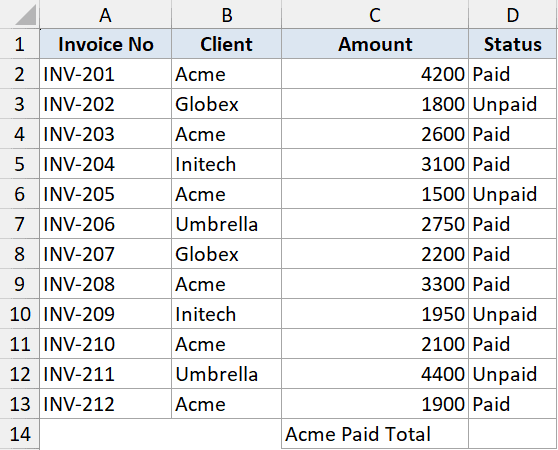
Here’s a set of freelancer invoices, each tagged with a client and a paid or unpaid status.

First I spill out every Acme invoice that’s been paid, into helper column F:

=FILTER(C2:C13,(B2:B13="Acme")*(D2:D13="Paid"))

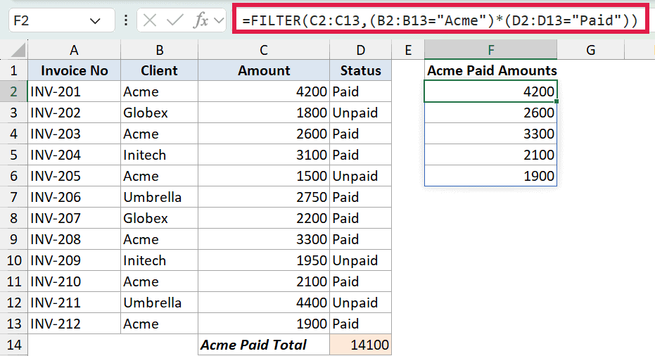
Then I total that spill range with SUBTOTAL. The F2# is a spill reference, which points at the whole spilled array and counts as a reference, so SUBTOTAL is happy:

=SUBTOTAL(9,F2#)

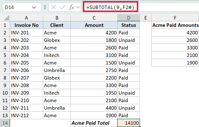
The result is 14,100, the total of Acme’s paid invoices. Swap the 9 for 3 to count them, 1 to average them, 4 for the largest, all over the same spilled range. That is how SUBTOTAL composes with dynamic arrays in modern Excel.

Tips & Common Mistakes

• SUBTOTAL ignores other SUBTOTAL formulas in its range. This is the most useful and least obvious thing about it. If your data already has subtotal rows mixed in, wrap a SUBTOTAL around the whole range and it won’t double-count. A regular SUM would, as Example 6 showed.
• Filtered rows are always ignored, period. No matter which function number you pick, if a filter has hidden a row, SUBTOTAL skips it. The 1-vs-101 distinction only changes what happens with rows hidden by hand.
• Hidden columns are always included. SUBTOTAL is built for vertical data. Hiding a column doesn’t change the result, regardless of function number.
• SUBTOTAL won’t take an array directly. It needs a reference, so =SUBTOTAL(9,FILTER(...)) errors. Spill the array into a range first and point SUBTOTAL at the spill reference, like =SUBTOTAL(9,F2#).
• Excel Tables give you SUBTOTAL for free. Convert your range to a Table and turn on the Total Row. Excel writes a =SUBTOTAL(109,...) for you, with a dropdown to switch operations.
• AGGREGATE is the modern cousin. Introduced in Excel 2010, AGGREGATE does everything SUBTOTAL does and adds the ability to also ignore errors. If your list has #DIV/0! errors, AGGREGATE handles them where SUBTOTAL can’t.
• Don’t confuse the function with the feature. Excel also has a Data then Subtotal button that inserts subtotal rows into a sorted list. That’s a separate workflow that writes SUBTOTAL formulas for you. This article is about the function itself.

In this article I covered the SUBTOTAL function from the everyday filtered total all the way to filter-aware conditional sums, a self-switching dashboard, and the dynamic array pattern for Excel 365.

The thread running through all of it is the same. SUBTOTAL only counts what you can see, and the function number decides exactly what that means.

I hope you found this article helpful.

List of All Excel Functions

Other Excel articles you may also like:

• Sum by Color in Excel