
If you have a long worksheet and want to tidy it up so you can collapse sections out of the way and focus on what matters, grouping rows is exactly what you need. Maybe you tried hiding rows, but then you lose the easy on-off toggle.
Grouping fixes that. It puts a little plus and minus button in the margin so you can fold whole blocks of rows up and open them back up in a click.
In this article, I’ll first show you a few ways to group rows in Excel (the manual method, Auto Outline, and Subtotal), and then how to collapse and expand those rows using the outline buttons, the level buttons, and the Hide Detail and Show Detail commands.
Method 1: Group Rows Manually
This is the approach you’ll use most of the time. You pick the rows you want to bundle together, and Excel adds a collapsible outline for them. It works no matter how your data is laid out.
Let’s suppose you have regional sales data, with a few cities listed under each region as shown below.
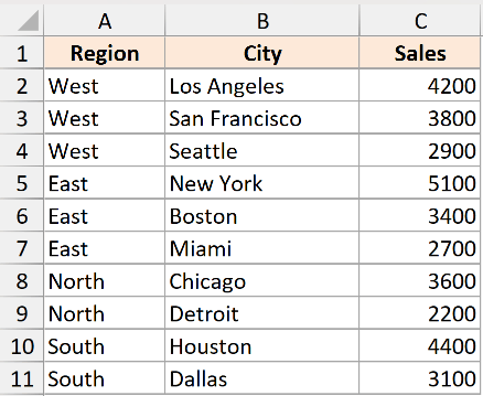
Say you want to group the city rows under the “West” region so you can collapse them when you don’t need the detail.
Here are the steps to group rows manually:
- Select the range you want to group. In this example, I have selected A2:A4
- Click the Data tab, and in the Outline group, click Group, then choose Group.
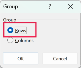
- In the Group dialog box, select Rows and click OK.
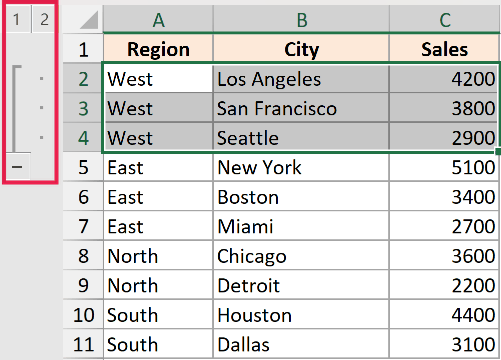
Excel adds an outline bar in the left margin that spans the rows you selected, along with a minus button you can click to collapse the group.
Pro Tip: Instead of going through the ribbon, select the rows and press Shift + Alt + Right Arrow to group them instantly. To ungroup, select the rows and press Shift + Alt + Left Arrow.
A quick note on selecting rows. If you only select a few cells instead of whole rows, Excel won’t know whether you mean rows or columns, so it shows the Group dialog box asking you to pick. Selecting full row numbers skips that question.
Creating Nested Groups
You can also group rows within a group, which is handy when your data has more than one level.
For example, you might group all the cities under a region, and then group several regions together inside a bigger group.
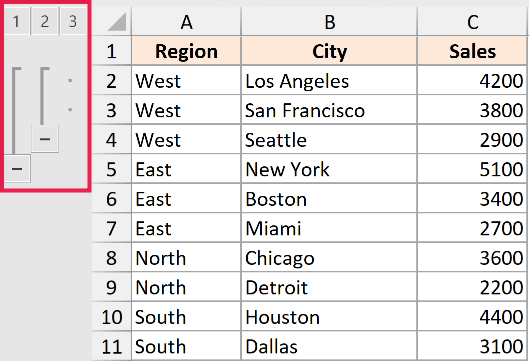
To do this, first group the smaller blocks of rows, then select a larger range that contains those groups and run Group again. Excel stacks the outline bars so you get a second level, and you’ll see the outline buttons go up to 1, 2, 3.
Method 2: Group Rows Automatically with Auto Outline
If your worksheet already has summary formulas, like a total row under each region built with SUM or SUBTOTAL, Excel can build the entire outline for you in one click.
This works because Auto Outline reads your formulas to figure out which rows are detail and which are summaries. No formulas means Excel has nothing to go on, so it won’t be able to create the outline.
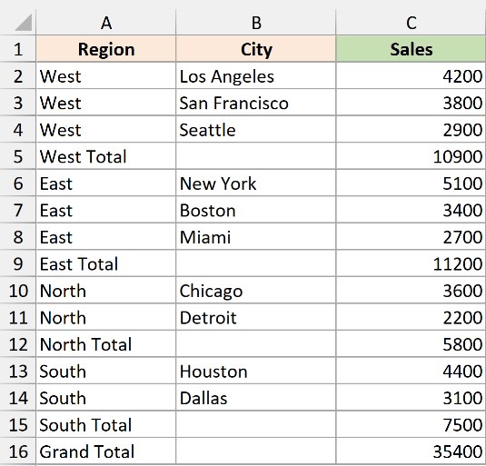
Let’s suppose you have sales data where each region has a total row below its cities, calculated with a SUM formula, plus a grand total at the bottom.
Here are the steps to group rows using Auto Outline:
- Click any cell inside your dataset.
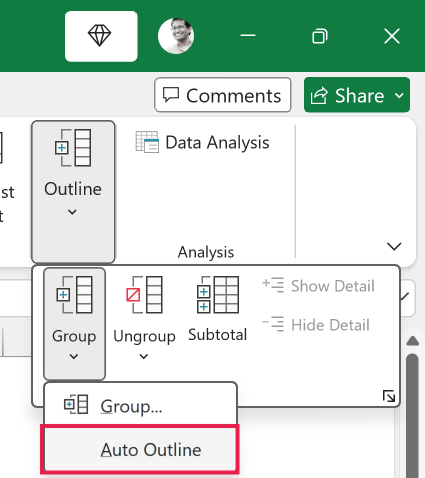
- Click the Data tab, in the Outline group click the Group dropdown arrow, then choose Auto Outline.
Excel reads your summary formulas and adds outline bars for every group automatically.
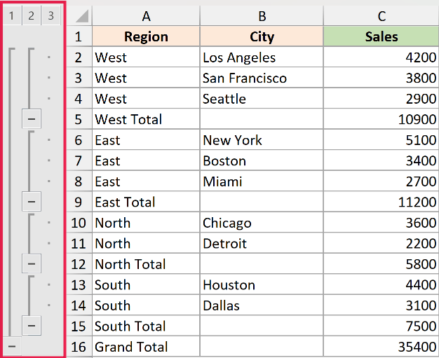
You can then collapse and expand them just like you would with a manual group.
Method 3: Group Rows Using Subtotal
The Subtotal feature does two jobs at once. It inserts subtotal rows into your data and groups the detail rows underneath them at the same time, so you get a ready-made outline.
This is the one to reach for when you want totals broken out by category and a collapsible view of the same data.
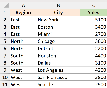
Let’s suppose you have a list of sales sorted by region, and you want a subtotal for each region.
Here are the steps to group rows with Subtotal:
- Make sure your data is sorted by the column you want to group by (in this case, Region), then click any cell in the dataset.
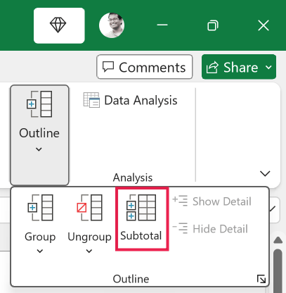
- Click the Data tab, and in the Outline group, click Subtotal.
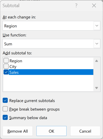
- In the Subtotal dialog box, set “At each change in” to Region, set “Use function” to Sum, and check the Sales option under “Add subtotal to”. Then click OK.
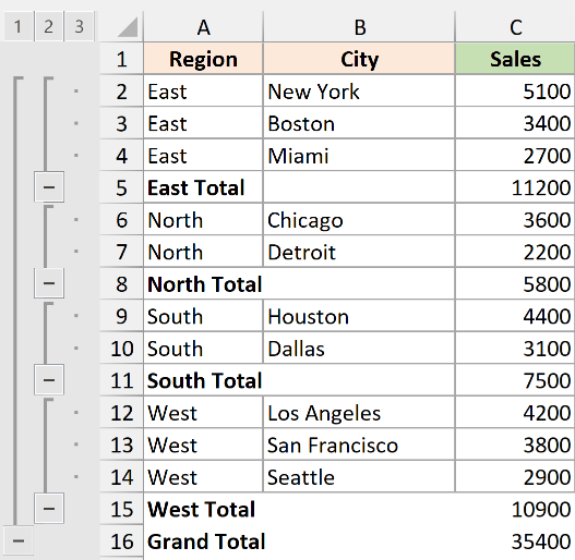
Excel adds a subtotal row after each region and a grand total at the bottom. It also groups the detail rows for you, so you get the same plus and minus outline buttons in the margin.
How to Collapse and Expand Grouped Rows
Once your rows are grouped (using any of the three methods above), Excel shows outline controls in the left margin next to the row numbers.
This is where collapsing comes in. Collapsing simply folds the detail rows out of sight so you’re left with the summary, and nothing is deleted.
The controls are the plus and minus buttons, the numbered level buttons, and a pair of ribbon commands. Let me walk through each one.
Collapse and Expand With the Plus and Minus Buttons
This is the part you’ll use most. Each group has a minus button (−) in the outline margin, and once you collapse it, that button turns into a plus button (+) so you always know where the hidden rows are.
Here are the steps to collapse a single group of rows:
Click the minus button (−) in the outline margin next to the group you want to hide.
The detail rows fold away and you’re left with just the subtotal (or summary) row for that group.
To bring the rows back, click the plus button (+) next to the collapsed group.
The hidden detail rows come straight back into view. You can collapse and expand the same group as many times as you like without losing anything.
Collapse or Expand Everything With the Level Buttons
Clicking the plus and minus buttons one by one is fine for a row or two.
But when you want to collapse or expand the whole sheet at once, the level buttons are much faster.
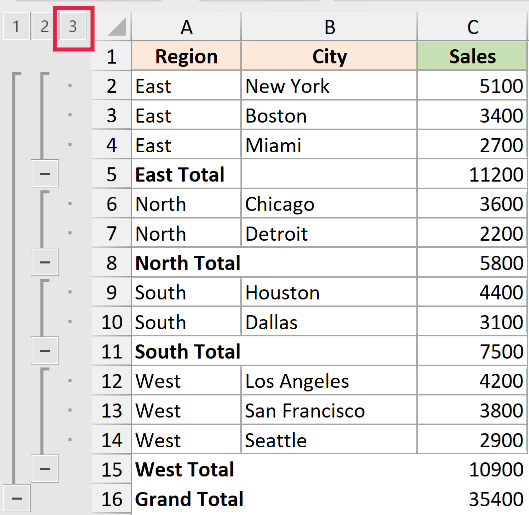
These are the small numbered buttons (1, 2, 3) at the very top-left of the outline margin, just above the row numbers. Each number shows a different amount of detail.
Here is what each level does with our region example:
- Level 1 shows only the top line, like the grand total. Everything else is collapsed.
- Level 2 shows the next layer down, so you’d see the region subtotal rows but not the individual detail rows.
- Level 3 expands everything, including all the detail rows under each region.
The exact numbers you see depend on how many levels of grouping your data has. A simple table with one layer of groups gives you just a 1 and a 2.
To collapse the whole sheet down to the summary level click the 2 button at the top-left of the outline margin to show only the subtotal rows.
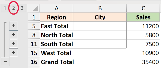
Every group collapses at the same time, and you see a clean summary view without touching each minus button.
To expand everything again, click the highest level number (for example, 3) and all the detail rows reappear across the entire sheet in one click.
Collapse and Expand Using Hide Detail and Show Detail
If you’d rather not hunt for the small plus and minus buttons, Excel gives you the same actions as proper buttons on the ribbon.
They do exactly what the plus and minus buttons do.
Here are the steps to collapse a group from the ribbon:
- Select a cell in the group of rows you want to collapse, then click the Data tab and, in the Outline group, click Hide Detail.
The detail rows for that group collapse, just as if you had clicked the minus button.
To expand the rows again, select a cell in the collapsed summary row, then click the Data tab and click Show Detail in the Outline group. The hidden rows come right back.
Pro Tip: If the outline margin and its buttons are not showing at all, press Ctrl + 8 to toggle the outline symbols back on.
How to Ungroup Rows and Remove the Outline
If you no longer need a group, you can take it apart without deleting any of your data.
To ungroup specific rows, select those rows, click the Data tab, and in the Outline group click Ungroup, then choose Ungroup.
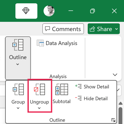
The outline bar for that section disappears. You can also press Shift + Alt + Left Arrow to do the same thing.
If you want to clear every group on the sheet at once, click any cell in the data, then click the Data tab, click the Ungroup dropdown arrow in the Outline group, and choose Clear Outline.
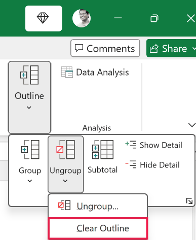
This wipes the entire outline in one step, but it leaves all of your rows in place.
Pro Tip: If you used Subtotal to create your groups and want to remove both the subtotal rows and the outline, open the Subtotal dialog box again (Data tab, Subtotal) and click Remove All.
Things to Keep in Mind
- Collapsing is not the same as hiding rows. When you hide rows the normal way (right-click and choose Hide), there’s no visible marker, so it’s easy to forget the rows are even there. Collapsed rows always keep the plus and minus control in the margin, which makes them easy to spot and bring back.
- Collapsed rows stay collapsed when you save. If you save and close the file with groups collapsed, they’ll still be collapsed when you reopen it. So you can set up a clean summary view and hand the file off as-is.
- Excel prints what’s on screen. If rows are collapsed, they won’t appear in the printout, so expand everything first if you need the full data on paper.
- Summary rows are expected below the detail. By default Excel puts the collapse button at the bottom of each group. If your totals sit above the detail rows instead, your groups can look upside down. To fix this, click the Data tab, click the small dialog box launcher in the corner of the Outline group, and uncheck “Summary rows below detail”.
- Auto Outline only works with summary formulas. If you try it on plain data with no totals or SUM formulas, Excel can’t detect any structure and won’t create an outline. Use the manual method for plain data.
- Subtotal needs your data sorted first. If the regions are scattered around, Subtotal will create a separate subtotal every time the value changes, which gives you a messy result. Sort by the grouping column first, then run Subtotal.
- Ungrouping removes the outline only, not your rows. So if you ungroup, none of your actual data is deleted. The same is true for Clear Outline. It just removes the grouping, leaving all rows in place.
In this article, I showed you how to group rows in Excel manually, with Auto Outline, and with Subtotal, and then how to collapse and expand them using the plus and minus buttons, the level buttons, and the Hide Detail and Show Detail commands, plus how to remove the outline when you’re done.
I hope you found this article helpful.


