

If you want to swap out specific text inside your cells, like turning every dash in a phone number into nothing or changing “Street” to “St”, the SUBSTITUTE function is what you need.
A lot of people reach for Find and Replace, but that changes your data permanently and can’t run down a whole column live as the data changes. SUBSTITUTE does it with a formula, so the original stays put and the result updates on its own.
In this article, I’ll show you how to use SUBSTITUTE in Excel with six practical examples, from cleaning phone numbers to replacing only a specific occurrence of a word.
SUBSTITUTE Function Syntax and Arguments
SUBSTITUTE replaces specific text in a string with new text you choose. It looks for the actual characters you name, not a position in the cell.
Here is the syntax:
=SUBSTITUTE(text, old_text, new_text, [instance_num])
Here is what each argument means:
- text – The text (or the cell holding it) you want to change.
- old_text – The text you want to find and replace.
- new_text – The text you want to put in its place.
- instance_num – (Optional) Which occurrence of old_text to replace. Leave it out and every occurrence gets replaced.
Pro Tip: SUBSTITUTE is case-sensitive. “St” and “st” are treated as two different things, so make sure old_text matches the exact case in your cells.
SUBSTITUTE works in every modern version of Excel, including Excel 2019, 2021, 2024, Microsoft 365, and the web version.
Example 1: Remove Dashes From Phone Numbers Using SUBSTITUTE
Let’s start with a common cleanup job. Below I have a list of phone numbers in column A that were entered with dashes, and I want a clean version with the dashes removed.
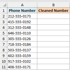
Here is the formula:
=SUBSTITUTE(A2:A11,"-","")
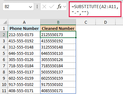
I gave old_text a dash and new_text an empty string (“”), which tells Excel to remove the dashes instead of swapping them for something.
If you’re on Microsoft 365 or Excel 2021 and later, one formula in the top cell fills the whole column on its own. This is called a spill, and you don’t need to drag anything down.
On Excel 2019 or older, write it for the first row as =SUBSTITUTE(A2,"-","") and copy it down the column instead.
Example 2: Replace a Word Using SUBSTITUTE (Street to St)
Now let’s swap one word for another. Below I have a list of street addresses in column A, and I want to shorten the word “Street” to “St” in each one.
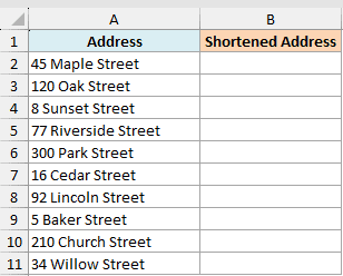
Here is the formula:
=SUBSTITUTE(A2:A11,"Street","St")
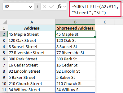
Excel finds “Street” in each address and replaces it with “St”, leaving the house number and everything else untouched.
The single formula in the top cell spills the cleaned addresses down the whole column in Microsoft 365 and Excel 2021 or later.
Remember the case rule here. “Street” will not match “street” with a lowercase s, so type old_text exactly as it appears in your data.
Example 3: Remove All Spaces From Text Using SUBSTITUTE
Sometimes you need text with no spaces at all, like turning a name into a username or cleaning up a code. Below I have a list of full names in column A, and I want to remove every space.

Here is the formula:
=SUBSTITUTE(A2:A11," ","")
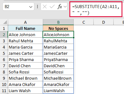
Here old_text is a single space and new_text is an empty string, so every space in the name gets stripped out.
This removes all spaces, including the ones in the middle. If you only want to trim spaces from the start and end, use the TRIM function instead, which keeps single spaces between words.
Example 4: Replace Only the Nth Occurrence Using instance_num
This is where SUBSTITUTE does something Find and Replace can’t. You can tell it to change only one specific occurrence of the text and leave the rest alone.
Below I have a list of file paths in column A. Each uses a dash as a separator, and I want to replace only the second dash with a slash, keeping the first dash as is.
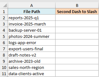
Here is the formula:
=SUBSTITUTE(A2:A11,"-","/",2)
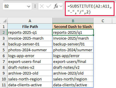
The 4th argument (instance_num) is set to 2, so Excel replaces only the second dash and leaves the first one alone. Change it to 1 and it would swap only the first dash.
This is the answer to “what is instance number in SUBSTITUTE”. It’s simply which occurrence you want to target, counting from the left. Leave it out and every occurrence gets replaced.
Example 5: Substitute Multiple Characters Using Nested SUBSTITUTE
SUBSTITUTE only handles one piece of text per call, but you can nest several together to clean up multiple characters at once. Below I have a list of product codes in column A with slashes and dots mixed in, and I want to remove both.
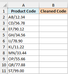
Here is the formula:
=SUBSTITUTE(SUBSTITUTE(A2:A11,"/",""),".","")
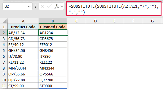
The inner SUBSTITUTE removes the slashes first. That cleaned text is then passed to the outer SUBSTITUTE, which removes the dots. You can keep nesting more layers to strip additional characters.
Read it from the inside out. The result of each SUBSTITUTE becomes the text argument for the next one wrapped around it.
Example 6: Count How Many Times a Character Appears
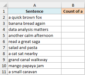
You can use SUBSTITUTE for a handy counting trick too. Below I have a list of sentences in column A, and I want to count how many times the letter “a” appears in each one.
Here is the formula:
=LEN(A2)-LEN(SUBSTITUTE(A2,"a",""))
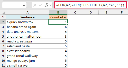
The idea is simple. LEN measures the original length, then you measure the length again after SUBSTITUTE removes every “a”. The difference tells you how many “a” characters were there, a neat way to count characters in Excel.
I’ve kept this one as a per-row formula that you copy down, since it reads more clearly that way. Remember it counts lowercase “a” only, because SUBSTITUTE is case-sensitive.
SUBSTITUTE vs REPLACE: What’s the Difference?
These two functions sound similar but work in opposite ways, and mixing them up is a common mistake.
- SUBSTITUTE replaces text by matching the actual characters. You tell it what text to find, and it swaps every match (or a specific one) regardless of where it sits.
- REPLACE replaces text by position. You tell it to start at character 3 and change the next 4 characters, without caring what those characters are.
Use SUBSTITUTE when you know the text you want to change, like a word or a symbol. Use the Excel REPLACE Function when you know the exact position in the string, like the first three digits of a code.
Tips and Common Mistakes to Keep in Mind
A few things trip people up with SUBSTITUTE, so keep these in mind:
- It’s case-sensitive. old_text must match the exact case in your cell. To handle mixed case, nest SUBSTITUTE calls or pair it with the Excel UPPER Function or Excel LOWER Function first.
- To delete text, use an empty string. Set new_text to “” (two quotes with nothing between) and SUBSTITUTE removes old_text instead of replacing it.
- It doesn’t support wildcards. SUBSTITUTE looks for exact text, so
*and?are treated as literal characters, not wildcards. - The result is text. Even if the output looks like a number (a phone number with dashes removed), Excel treats it as text. Wrap it in VALUE if you need a real number.
Wrapping It Up
That’s how the SUBSTITUTE function works in Excel. We used it to clean phone numbers, swap words, strip spaces, replace a specific occurrence with instance_num, remove multiple characters with nesting, and even count how often a character shows up.
Once you get comfortable with the four arguments, it becomes one of the handiest text functions for cleaning up messy data. I hope you found this tutorial helpful.
Other Excel Articles You May Also Like:
