

If you want to count rows that meet more than one condition at the same time, like how many laptops the East region sold, a plain count won’t get you there. You need a way to check two or more criteria at once and only count the rows where all of them are true.
That’s exactly what the COUNTIFS function does. In this article, I’ll show you how to use COUNTIFS in Excel with clear examples, covering multiple criteria, comparison operators, number and date ranges, OR logic, wildcards, and how it differs from COUNTIF.
Follow along with the example file
COUNTIFS Function Examples.xlsx
When to Use the Excel COUNTIFS Function
Use COUNTIFS when you want to count cells that meet a single criterion or several criteria across different ranges. It only counts a row when every condition you set is met.
It’s the go-to function for questions like “how many orders were from the East region AND above 100 units” or “how many sign-ups happened between two dates on a specific plan.”
COUNTIFS Function Syntax
Here is the syntax of the COUNTIFS function:
=COUNTIFS(criteria_range1, criteria1, [criteria_range2, criteria2]...)
- criteria_range1 – the first range of cells you want to check against criteria1.
- criteria1 – the condition to check in criteria_range1 (a number, text, expression, or cell reference).
- [criteria_range2, criteria2] – optional extra range and condition pairs. You can add up to 127 pairs in total.
A cell is counted only when it satisfies every criteria pair you give it. Each extra range must have the same number of rows and columns as criteria_range1, otherwise Excel returns an error.
Pro Tip: Any criteria that uses text or a comparison symbol (such as =, >, <, >=) must be wrapped in double quotes, like “East” or “>100”.
Example 1: Count Cells That Meet Multiple Criteria
Let’s start with the most common use of COUNTIFS: counting rows that match two conditions.
Below I have a dataset of sales orders. Each row has a sales rep, their region, the product sold, and the number of units. I want to count how many orders James made in the East region.
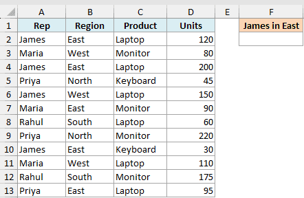
Here is the formula:
=COUNTIFS(A2:A13,"James",B2:B13,"East")
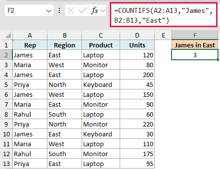
This returns 3, because three orders have James in column A and East in column B at the same time.
The first pair (A2:A13, “James”) finds the rep, and the second pair (B2:B13, “East”) finds the region. COUNTIFS only counts a row when both are true, so an order by James in the West is left out.
Example 2: Use Comparison Operators in the Criteria
COUNTIFS isn’t limited to exact matches. You can use comparison operators like greater than, less than, or not equal to inside the criteria.
Using the same sales dataset, I want to count how many laptop orders were above 100 units.
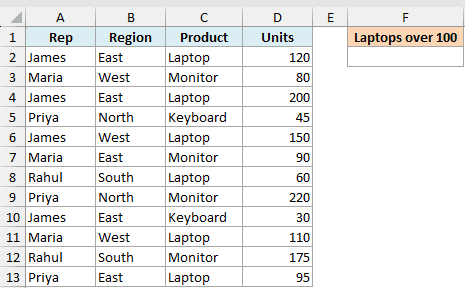
Here is the formula:
=COUNTIFS(D2:D13,">100",C2:C13,"Laptop")
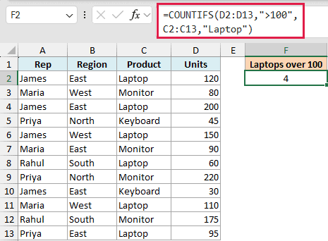
This returns 4. The first pair (D2:D13, “>100”) keeps only the rows above 100 units, and the second pair (C2:C13, “Laptop”) keeps only laptops.
Notice the operator sits inside the double quotes with the value: “>100”. You can do the same with “>=100”, “<50”, or “<>Laptop” to count everything that is not a laptop.
Example 3: Reference a Cell in the Criteria
Typing values straight into the formula works, but it’s often better to point the criteria at a cell. That way you can change the condition without editing the formula.
Here I’ve put the region I want in cell G2 and the minimum units in cell G3, with their labels sitting in column F. I want to count orders that match the region in G2 and have units greater than or equal to G3.
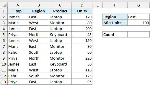
Here is the formula:
=COUNTIFS(B2:B13,G2,D2:D13,">="&G3)
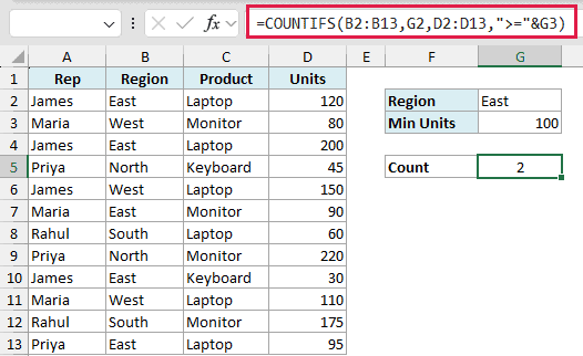
With East in G2 and 100 in G3, this returns 2.
When your criteria is just a cell reference (like G2), you use it directly. When you need an operator with a cell, you join them with the ampersand: “>=”&G3. Excel builds the text “>=100” behind the scenes, so keep the operator in quotes and the cell outside.
Follow along with the example file
COUNTIFS Function Examples.xlsx
Example 4: Count Values in a Number Range
A common need is counting numbers that fall between two values. COUNTIFS handles this by pointing two criteria at the same range, one for the lower bound and one for the upper bound.
Using the sales dataset again, I want to count how many orders had units between 50 and 150.
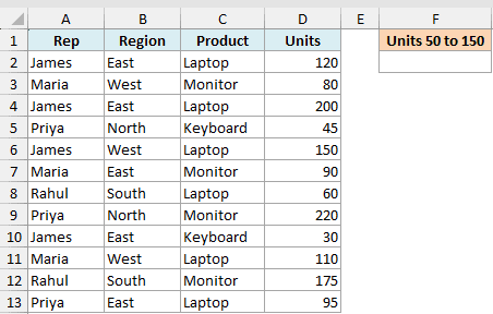
Here is the formula:
=COUNTIFS(D2:D13,">=50",D2:D13,"<=150")
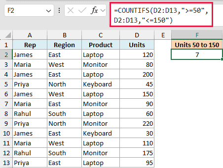
This returns 7. The trick is that both criteria ranges are the same column, D2:D13. The first checks for 50 or more, the second checks for 150 or less, and only orders that pass both are counted.
Example 5: Count Dates Between Two Dates
The same two-criteria trick works for dates. You can count records that fall inside a date window by setting a start date and an end date on the date column.
Below I have a table of new sign-ups with the date each person joined and the plan they picked. I want to count how many people signed up in February 2026.
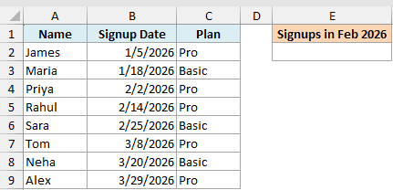
Here is the formula:
=COUNTIFS(B2:B9,">="&DATE(2026,2,1),B2:B9,"<="&DATE(2026,2,28))
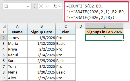
This returns 3 for these date-only values. The upper bound is midnight at the start of February 28, so timestamps later that day would be excluded.
I’ve used the DATE function to build each date so the formula doesn’t depend on your regional date format. You could also point these at cells holding the start and end dates, using “>=”&F1 and “<=”&F2.
Pro Tip: Need the count for a specific plan in that window too? Just add another pair, like C2:C9,”Pro”, and COUNTIFS will only count February sign-ups on the Pro plan.
Example 6: Use Wildcards for Partial Matches
When you want to match part of a text value instead of the whole thing, wildcards come in handy. COUNTIFS supports two of them: the question mark (?) matches any single character, and the asterisk (*) matches any sequence of characters.
Back in the sales dataset, I want to count orders where the product name ends in “or” (that’s Monitor) and the units are above 100.
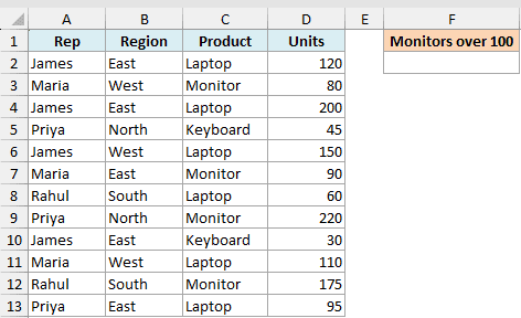
Here is the formula:
=COUNTIFS(C2:C13,"*or",D2:D13,">100")
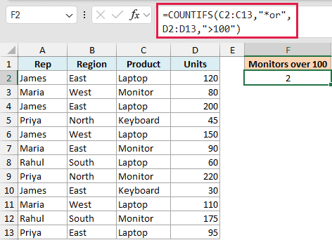
This returns 2. The pattern “*or” matches any product ending in “or”, so it picks up every Monitor, and the second pair keeps only the ones above 100 units.
If you ever need to match a literal question mark or asterisk in your text, put a tilde (~) in front of it, like “~?” to find an actual question mark.
Example 7: COUNTIF vs COUNTIFS: What’s the Difference?
This one trips up a lot of people, so it’s worth clearing up. COUNTIF (no S) counts with a single criterion. COUNTIFS (with an S) counts with one or more criteria at once.
Using the sales dataset, counting all East orders is a single-criterion job, so COUNTIF is enough:
=COUNTIF(B2:B13,"East")
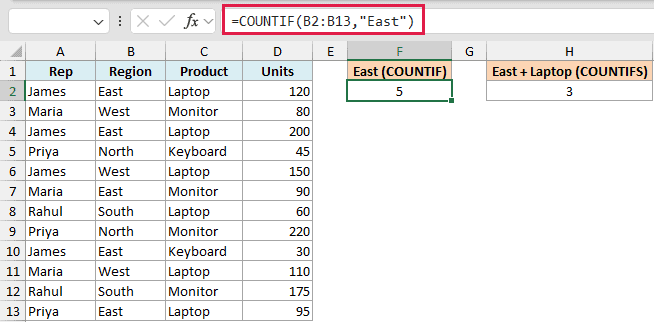
This returns 5. The moment you want to add a second condition, like East orders that were also laptops, you switch to COUNTIFS:
=COUNTIFS(B2:B13,"East",C2:C13,"Laptop")
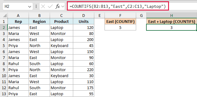
This returns 3. COUNTIFS can handle a single criterion too, so if you’re unsure how many conditions you’ll end up needing, you can just start with COUNTIFS and add pairs as you go. For a full walkthrough, see the Excel COUNTIF Function tutorial.
Example 8: Count Per Category With a Spilling Formula
COUNTIFS returns a single number on its own. But in Microsoft 365, Excel 2024, Excel 2021, or Excel for the web, you can pair it with the UNIQUE function to get a count for every category at once, spilling down the column automatically.
Using the sales dataset, I want a count of orders for each region without typing a separate count formula for each one. The region labels in column F come from =UNIQUE(B2:B13); the formula below returns the counts in column G.
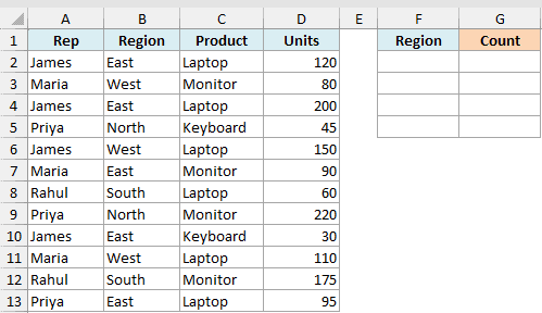
Here is the formula:
=COUNTIFS(B2:B13,UNIQUE(B2:B13))
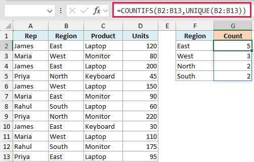
UNIQUE pulls the distinct regions (East, West, North, South), and COUNTIFS counts each one, returning 5, 3, 2, and 2. The result spills into the cells below on its own, so you don’t drag or copy anything down.
This spilling version works in Microsoft 365, Excel 2024, Excel 2021, and Excel for the web. On Excel 2019 or earlier, list your categories in a column first, then use a regular COUNTIFS next to each and fill it down.
Example 9: Count With OR Logic (East or West)
COUNTIFS combines its criteria with AND. To count rows that match one value OR another in the same column, you can give it a list of values.
Using the same sales dataset, I want to count orders from either the East or the West region.
Here is the formula:
=SUM(COUNTIFS(B2:B13,{"East","West"}))
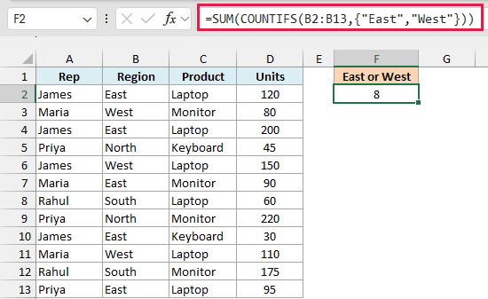
This returns 8. The curly braces hold an array constant, so COUNTIFS counts East (5) and West (3) separately and returns both numbers. SUM adds them to give one total.
This works in all Excel versions without Ctrl+Shift+Enter, and you can add more regions inside the braces. There’s no double counting for East or West because a cell can’t hold both regions.
Things to Keep in Mind
A few points that save time and avoid errors when working with COUNTIFS:
- All the criteria ranges must be the same size. If criteria_range1 is 12 rows, every other range must also be 12 rows, or Excel returns a #VALUE! error.
- Criteria are not case-sensitive. “East” and “east” are treated as the same value.
- Wrap text and operators in double quotes, but use a cell reference on its own without quotes.
- You can use OR logic by adding two COUNTIFS results. For values in one column, see Example 9’s array constant method. When the two conditions are on different columns, a row that meets both gets counted twice.
- If a criteria points to an empty cell, COUNTIFS treats that empty cell as a 0.
- COUNTIFS has sibling functions that use the exact same criteria style. Use the Excel SUMIFS Function to add values on multiple criteria, and the Excel AVERAGEIFS Function to average them.
That covers the main ways to use the COUNTIFS function in Excel, from simple two-criteria counts to number ranges, date ranges, wildcards, and the modern spilling version. Once you get comfortable pairing ranges with criteria, you can answer almost any “how many rows match all of these conditions” question in one formula. I hope you found this tutorial helpful.
Other Excel Articles You May Also Like:
- How to Use Multiple Criteria in Excel COUNTIF and COUNTIFS Function
- How to Count Cells that Contain Text Strings
- Count Cells Less than a Value in Excel (COUNTIF Less Than)
- Count Between Two Numbers in Excel (COUNTIF / COUNTIFS)
- Excel Wildcard Characters – What are these and How to Best Use it
- How to Use Excel COUNTBLANK Function
- IF AND in Excel
- Difference Between SUMIF and SUMIFS
