

If you want to add up only the numbers that meet one condition, like the total sales for a single region, you cannot use a plain SUM because SUM adds everything.
But nothing to worry about. This is exactly what the SUMIF function is built for, and it’s easy once you see it in action.
In this article, I’ll show you how to use SUMIF in Excel with simple examples, from a basic category total to comparison operators, text and wildcards, and a modern one-formula version that sums every category at once.
Follow along with the example file
SUMIF Function Examples.xlsx
What the SUMIF Function Does
SUMIF adds the numbers in a range, but only for the rows where your one condition is true.
Think of a sales table where you want the total for just the North region. SUMIF looks down the region column, finds every North row, and adds up only those amounts.
It handles a single condition. When you need two or more conditions at once (say North region AND laptops), you move up to the SUMIFS function, which I’ll point out again later.
SUMIF Function Syntax and Arguments
Here is the syntax of the SUMIF function:
=SUMIF(range, criteria, [sum_range])
SUMIF takes three arguments, with range and criteria required and sum_range optional.
- range (required): the cells you want Excel to check against your condition.
- criteria (required): the condition itself, like
"North",">1000", or a cell reference. - sum_range (optional): the cells that actually get added. Leave it out and Excel adds the
rangecells instead.
The important thing to notice is that sum_range is the last argument, and it’s optional.
This is the opposite of SUMIFS, where the sum range comes first. If you jump between the two functions, this is the number one thing that trips people up.
Pro Tip: In SUMIF the sum range is last and optional. In SUMIFS it’s first and required. Mixing up the order is the most common SUMIF/SUMIFS mistake.
Example 1: How to Use SUMIF to Sum by Category
Let’s start with the most common use, adding up the amounts for one category.
Below is a small sales dataset. Column A has the region, column B the product, and column C the sale amount. I want the total amount for the North region.
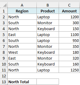
Here is the formula:
=SUMIF(A2:A11,"North",C2:C11)
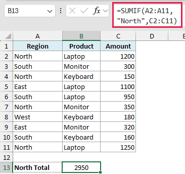
This gives you 2950.
Excel scans the region column (A2:A11), finds every row where it says North, and then adds up the matching amounts from column C. The text criteria "North" goes in double quotes.
Example 2: Using SUMIF with Comparison Operators (Greater Than, Less Than)
You can also sum based on a number condition instead of matching text.
Here I want the total of all sales that are greater than 1000. I’m using the same dataset, with the amounts in column C.
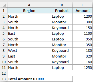
Here is the formula:
=SUMIF(C2:C11,">1000")
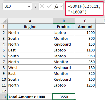
This returns 3550.
Notice there’s no sum_range here. Since I’m checking the same column I want to add, I can leave the third argument out and SUMIF adds the range cells directly.
The operator and number sit inside one set of quotes as ">1000". You can use ">", "<", ">=", "<=", and "<>" (not equal to) the same way.
Example 3: Using SUMIF with Text and Wildcards
SUMIF can match partial text using wildcards, which is handy when your labels share a common start or contain a word.
The two wildcards are the asterisk * (any number of characters) and the question mark ? (exactly one character).
Below is the same dataset. This time I want the total for every product whose name starts with “Key”, which covers all the keyboards.
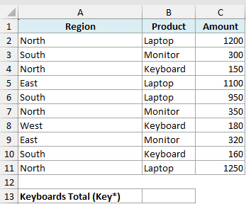
Here is the formula:
=SUMIF(B2:B11,"Key*",C2:C11)
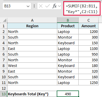
This gives you 490.
The * after Key tells Excel to match anything that begins with those letters. To match text that appears anywhere, you’d wrap it in asterisks, like "*book*".
Pro Tip: To match a real asterisk or question mark as a character, put a tilde in front of it (~* or ~?). Otherwise Excel treats them as wildcards.
Follow along with the example file
SUMIF Function Examples.xlsx
Example 4: When the Sum Range Is Different from the Criteria Range
In the first example the condition and the numbers happened to be handled by separate columns already. Here I want to make that split obvious, because it’s where sum_range really earns its place.
I’m using the same table. I want the total amount for the Laptop product. So my condition looks at the product column (B), but the numbers I add come from the amount column (C).
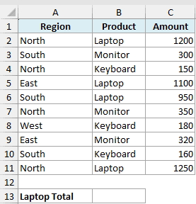
Here is the formula:
=SUMIF(B2:B11,"Laptop",C2:C11)
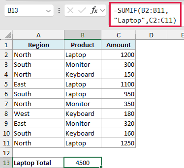
This returns 4500.
The range (B2:B11) is where Excel checks the condition, and the sum_range (C2:C11) is the separate column it adds. Keep both ranges the same height so the rows line up correctly.
Example 5: Referencing a Cell in the Criteria
Typing the condition straight into the formula works, but hard-coding "North" or "Laptop" means editing the formula every time you want a different region.
A cleaner approach is to put the condition in a cell and point the criteria at that cell. Here I’ve typed South in cell E2, and I want the total for whatever region is sitting in E2.
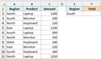
Here is the formula:
=SUMIF(A2:A11,E2,C2:C11)
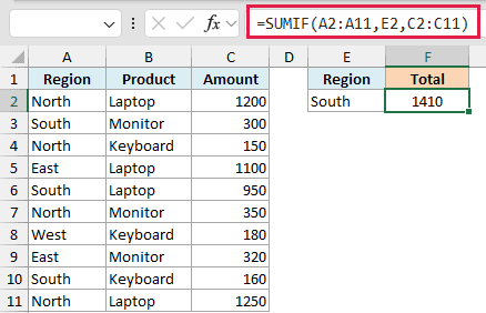
With South in E2, this gives you 1410.
Now you can change the region in E2 and the total updates on its own. This is the trick to build a quick lookup where someone picks a region and instantly sees its total.
When you combine a cell reference with an operator, join them with &, like ">"&E2 to sum everything greater than the value in E2.
Example 6: Sum Every Category at Once with UNIQUE (Modern Excel)
A single SUMIF returns one number. If you have four regions, the older way was to write the formula once and copy it down next to a list of region names.
In Microsoft 365 you can do the whole thing with one formula. Feeding SUMIF a list of the unique regions makes it spill a separate total for each one.
Below is the same dataset. I want a total for every region, all from one formula.
First, enter =UNIQUE(A2:A11) in E2 to spill the region names.
Then enter the formula below in F2 to get the matching totals.
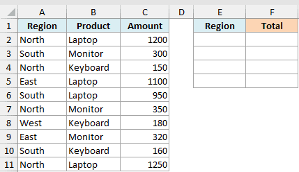
Here is the formula:
=SUMIF(A2:A11,UNIQUE(A2:A11),C2:C11)
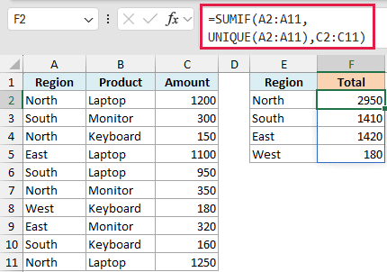
UNIQUE pulls the distinct region names (North, South, East, West), and SUMIF returns a total for each. The results spill down automatically, so you get 2950, 1410, 1420, and 180 without copying anything.
This works in Microsoft 365, Excel 2024, Excel 2021, and Excel for the web, where dynamic arrays and UNIQUE are available. In Excel 2019 or earlier you’d list the regions yourself and drag the SUMIF down beside them.
Example 7: Sum Expenses On or After a Date
You can use SUMIF to total expenses on or after a date. This is handy when you only want expenses from a certain day onward.
Below are office expenses, with dates in column A, expense types in B, and amounts in C. The goal is to total expenses from September 15, 2026 onward.
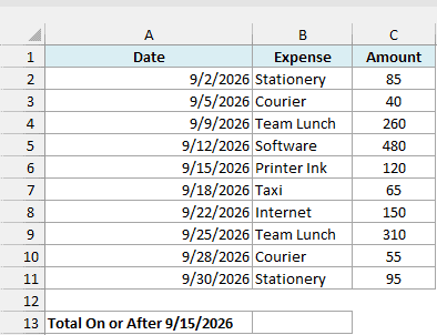
Here is the formula:
=SUMIF(A2:A11,">="&DATE(2026,9,15),C2:C11)
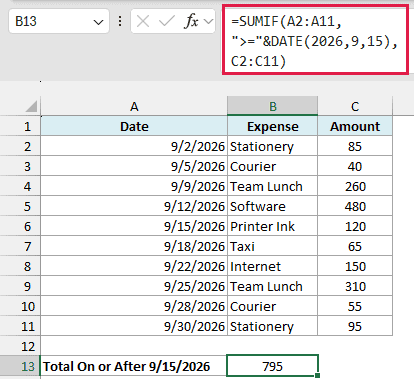
This returns 795.
The ">=" is joined with & to DATE(2026,9,15), which builds the date from its year, month, and day.
September 15 is included because >= means on or after, so the total includes the 120 for Printer Ink.
Typing ">=9/15/2026" depends on your computer’s date settings. Using DATE avoids that problem, whatever regional date format your computer uses.
Example 8: Sum Based on Blank or Non-Blank Cells
Below is an invoice table with amounts in column C and Paid On dates in column D. A blank Paid On cell means the invoice is unpaid. Let’s total the unpaid invoices first, then the paid ones.
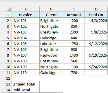
To total the unpaid invoices, where Paid On is blank, use this formula:
=SUMIF(D2:D11,"",C2:C11)
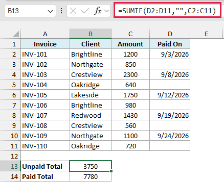
This returns 3750. The criteria "" means blank, with nothing between the two double quotes. SUMIF checks D2:D11 and adds the matching amounts from C2:C11.
For the paid invoices, where Paid On has a date, use this formula:
=SUMIF(D2:D11,"<>",C2:C11)
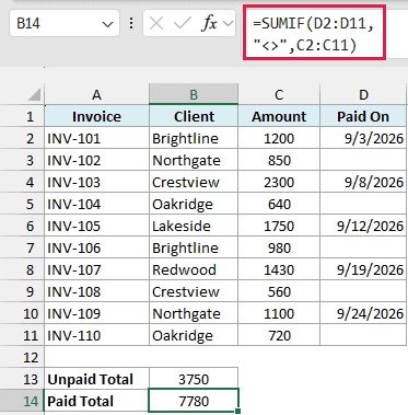
This returns 7780. The criteria "<>" means not equal to blank, so SUMIF adds the amounts for rows where Paid On isn’t empty.
When to Use SUMIFS Instead
SUMIF handles exactly one condition. The moment you need two or more at the same time, it’s the wrong tool.
Say you want the total for laptops in the North region only. That’s two conditions (product and region), so you’d use the SUMIFS function instead.
The same idea applies to counting. To count cells on one condition use COUNTIF function, and for multiple conditions use COUNTIFS function.
Tips and Common Mistakes
A few things to keep in mind so SUMIF behaves the way you expect:
- Watch the argument order versus SUMIFS. In SUMIF the sum range is last (
range, criteria, [sum_range]). In SUMIFS it comes first. This is the most common slip. - Text and operators need double quotes. Use
"North",">1000","<>Laptop". Plain numbers like100don’t need quotes. - Keep the ranges the same size. The
rangeandsum_rangeshould have the same number of rows, or the totals will line up against the wrong cells. - Wildcards only work on text.
*and?match text criteria. They do nothing against numbers. - Blank cells are ignored. Empty cells in the
sum_rangeare simply skipped. They don’t count as zero and don’t cause an error.
That’s how the SUMIF function works in Excel, from a basic category total to comparison operators, wildcards, and a one-formula version for every category at once. I hope you found this article helpful.
Other Excel Articles You May Also Like:
