

If you want to find out where a value sits in a list, which row or which column it lands on, the MATCH function is what you’re looking for. It hands you back the position as a number, not the value itself.
That number feels useless on its own, but it’s the piece that powers two-way lookups and the classic INDEX MATCH combo. In this article I’ll walk through what MATCH does, the match_type argument that trips most people up, and several examples you can copy.
Follow along with the example file
MATCH Function Examples.xlsx
When to Use the MATCH Function in Excel
Use MATCH when you want the relative position of a value inside a row, a column, or a single-column list.
Feed it what you’re looking for and where to look, and it tells you the position number.
On its own that position isn’t the answer you want. Its real job is feeding that number into another function (most often INDEX) so you can pull back the matching value from somewhere else.
It sits in the lookup and reference group of Excel functions.
MATCH Function Syntax and Arguments
Here is the syntax of the MATCH function:
=MATCH(lookup_value, lookup_array, [match_type])
- lookup_value (required): The value you want to find the position of. It can be a number, text, a logical value, or a cell reference.
- lookup_array (required): The single row or single column of cells you’re searching through.
- [match_type] (optional): How Excel should match. It takes 0, 1, or -1, and it defaults to 1 if you leave it out.
The match_type is where people get burned, so here is what each one does:
- 0 finds the first value exactly equal to your lookup_value. The list can be in any order. This is the one you’ll use most.
- 1 (the default) finds the largest value less than or equal to your lookup_value. Your list must be sorted in ascending order.
- -1 finds the smallest value greater than or equal to your lookup_value. Your list must be sorted in descending order.
MATCH is not case-sensitive, and it returns the #N/A error when it can’t find a match.
Example 1: How to Find the Position of a Value (Exact Match)
Let’s start with the most common use: an exact match. Below I have a list of cities in column A, and I want to know the position of Tokyo in that list.
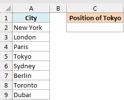
Here is the formula:
=MATCH("Tokyo", A2:A9, 0)
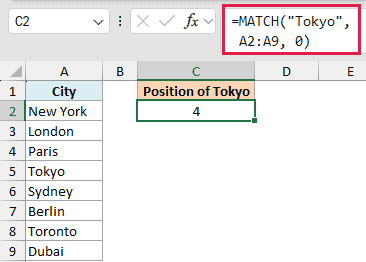
This returns 4, because Tokyo is the fourth city in the range A2:A9. The 0 as the last argument tells MATCH to look for an exact match, which is why the list doesn’t need to be sorted.
Since MATCH counts positions inside the range you give it, the number it returns is relative to that range, not to the worksheet row. Tokyo sitting in worksheet row 5 still returns 4 because A2 is position 1.
Pro Tip: When you use 0 for an exact match, MATCH returns the position of the first matching value it finds. If your list has duplicates, only the first one counts.
Example 2: Using MATCH Type 1 for an Approximate Match
Now let’s look at an approximate match. This is handy for tiers and brackets, where you want the band a value falls into rather than an exact hit.
Below I have a commission table sorted in ascending order. Column A holds the sales thresholds where each commission rate kicks in, and I want to find which band a sales figure of 6500 falls into.
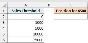
Here is the formula:
=MATCH(6500, A2:A6, 1)
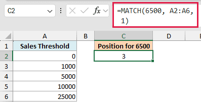
This returns 3. With match_type set to 1, MATCH finds the largest threshold that is still less than or equal to 6500. That’s 5000 in position 3, since 6500 hasn’t reached the 10000 threshold in position 4.
The catch with match_type 1 is that your list must be sorted in ascending order. If it isn’t, MATCH walks the list wrong and hands you back a position that makes no sense, with no error to warn you.
Pro Tip: Match_type defaults to 1, so leaving the third argument out gives you an approximate match on unsorted data and a silently wrong answer. Always type 0 when you want an exact match.
Example 3: How to Use INDEX and MATCH Together
A position number is rarely the end goal. Most of the time you want the value that sits at that position, which is exactly what INDEX MATCH does.
Below I have a table with employee names in column A and their departments in column B. I want to pull back the department for Priya without eyeballing the list.
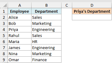
Here is the formula:
=INDEX(B2:B9, MATCH("Priya", A2:A9, 0))
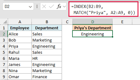
This returns Engineering. MATCH finds Priya’s position in column A, and INDEX uses that position number to grab the value from the same spot in column B.
Here MATCH returns 3 for Priya, then INDEX returns the third item in B2:B9. This combo is the reason MATCH exists for most people, and you can dig deeper in the guide on using Excel INDEX MATCH combo (with examples).
Example 4: How to Do a Two-Way Lookup with MATCH
Here is where MATCH really earns its keep. A two-way lookup finds a value at the intersection of a row and a column, using one MATCH for the row position and another for the column position.
Below I have a sales table. Salespeople run down column A, quarters run across row 1, and I want the number where James meets Q3.
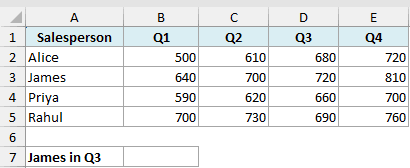
Here is the formula:
=INDEX(B2:E5, MATCH("James", A2:A5, 0), MATCH("Q3", B1:E1, 0))
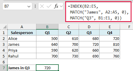
This returns 720. The first MATCH finds James in the row labels and gives 2, the second MATCH finds Q3 in the column labels and gives 3, and INDEX pulls the value from row 2, column 3 of the table.
The nice part is that both lookup values are flexible. Edit “James” or “Q3” in this formula to pull the new intersection. To change them from worksheet cells instead, replace those quoted values with cell references.
Example 5: Using MATCH with Wildcards
MATCH can also match on part of a text value using wildcards, as long as match_type is 0. The * stands for any number of characters and ? stands for a single character.
Below I have a list of product codes in column A, and I want the position of the code that ends in “-XL” without typing the whole thing.
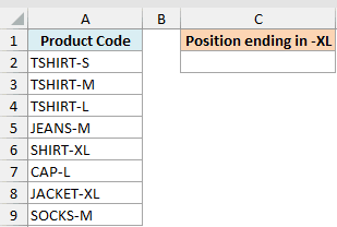
Here is the formula:
=MATCH("*-XL", A2:A9, 0)
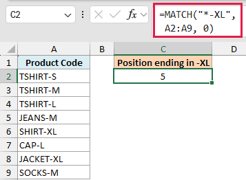
This returns 5, the position of the first code ending in “-XL”. The * before “-XL” tells MATCH to accept any characters ahead of it, so “SHIRT-XL” matches. You can read more about wildcard characters and how they behave.
Pro Tip: Wildcards only work with match_type 0. If your list itself contains a literal * or ?, put a tilde (~) in front of it in your lookup value so MATCH treats it as a normal character.
Example 6: Getting a Position for Several Values at Once (Dynamic Array)
In Excel for Microsoft 365, you can hand MATCH a whole range as the lookup_value and it returns a position for each one, spilling the results down the column. You don’t have to drag or copy the formula.
Below I have my city list in column A again, and a short list of cities to look up in column C. I want the position of each one.
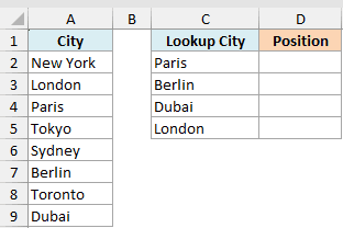
Here is the formula:
=MATCH(C2:C5, A2:A9, 0)
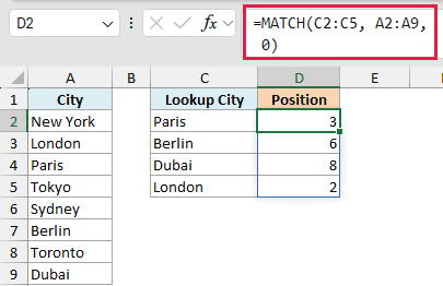
You type this once in the top cell and the results spill down automatically, one position for each city in C2:C5. It’s the fast way to look up a batch of values without filling a formula down manually.
This spilling behavior needs a dynamic-array version of Excel (Microsoft 365, Excel 2021 or later, or Excel for the web). Older Excel does not spill; use one lookup value per row and copy down with the lookup-list references fixed.
Tips and Common Mistakes to Keep in Mind
A few things that save headaches when you work with MATCH:
- Watch the default match_type. Leave the third argument out and you get 1 (approximate match), not an exact one. Type 0 whenever you want an exact match.
- Sort the list for match_type 1 or -1. Approximate matches assume the list is sorted (ascending for 1, descending for -1). Unsorted data gives a wrong position with no error.
- MATCH returns a position, not a value. If you want the value, wrap it in INDEX. The position alone is just a stepping stone.
- It’s not case-sensitive. “tokyo” and “TOKYO” match the same way. If you need a case-sensitive match, that takes a different approach, similar to making VLOOKUP case sensitive.
- Consider XMATCH if you have it. In Microsoft 365, Excel 2021, and Excel 2024, XMATCH is the modern successor to MATCH. It defaults to an exact match (no more match_type gotcha) and can search a list from the bottom up. It’s the match half of the newer XLOOKUP function.
MATCH looks simple, and it is, but the position it returns is the quiet workhorse behind INDEX MATCH and two-way lookups. Once the match_type argument clicks, you’ll reach for it far more than you’d expect. I hope you found this article helpful.
Other Excel Articles You May Also Like:
- Excel VLOOKUP Function
- Excel HLOOKUP Function
- Excel INDEX Function
- Excel INDIRECT Function
- Excel OFFSET Function
- VLOOKUP Vs. INDEX/MATCH
- Find the Closest Match of a Value in Excel
- Find the Last Occurrence of an Item in a List in Excel
- Get Unique Items from a List in Excel
- Lookup the Second, the Third, or the Nth Value in Excel
- INDEX MATCH with Multiple Criteria in Excel
