

If you want the average of only the numbers that meet one condition, like the average price of just your Accessories, the AVERAGEIF function is what you’re looking for.
A plain AVERAGE can’t do this, because it averages everything you give it and has no way to check a condition first.
AVERAGEIF returns a single value, but it also plays nicely with dynamic arrays. In Excel 365 or 2021 you can point it at a spilled range like =AVERAGEIF(A2#,">100") and it reads the whole spill.
In this article I’ll show you how to use AVERAGEIF in Excel, starting with a simple text condition and building up to numeric comparisons, wildcards, cell references, and averaging one column based on a condition in another.
AVERAGEIF Function Syntax
Here is what the AVERAGEIF function looks like:
=AVERAGEIF(range, criteria, [average_range])
Here is what each argument means:
- range is the group of cells Excel checks your condition against (like a column of categories or a column of numbers).
- criteria is the condition a cell has to meet to be included (like “Accessories”, “>100”, or a wildcard).
- [average_range] is optional. It’s the cells you actually want to average. If you leave it out, Excel averages the range itself.
Pro Tip: AVERAGEIF only checks one condition. If you need to average against two or more conditions at once (like Accessories that also sold more than 20 units), use the AVERAGEIFS function instead.
AVERAGEIF works in Excel for Microsoft 365, Excel 2024, 2021, 2019, 2016, and older versions back to 2007, plus Excel on the web and Excel for Mac.
When to Use AVERAGEIF in Excel
Use AVERAGEIF when you need to:
- Average the numbers in one category only (like the average price of one product type)
- Average only the values above or below a cutoff (like the average of scores of at least 40)
- Average a set of numbers while ignoring the zeros
- Average one column based on a condition sitting in another column
Let me show you a few practical examples of how this works.
Example 1: Average by Category With a Text Criteria
Let’s start with the most common use of AVERAGEIF.
Below is a product table with the product name in column A, the category in column B, the price in column C, and the units sold in column D.
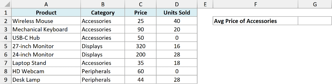
I want the average price of the products in the Accessories category.
Here is the formula:
=AVERAGEIF(B2:B9,"Accessories",C2:C9)
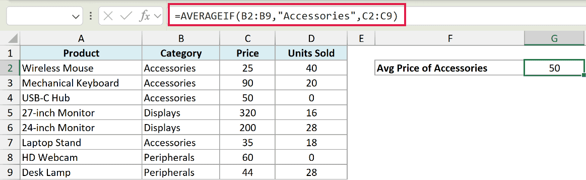
This gives me 50.
Excel looks down the category column (B2:B9), finds every row that says Accessories, and averages the matching prices in column C. Everything that isn’t Accessories is skipped.
Notice the text criteria “Accessories” is wrapped in double quotes. Any text you type straight into AVERAGEIF needs quotes around it.
Example 2: Average Values Above a Number
Here’s another common scenario, using a numeric condition instead of text.
I’m using the same product table: product in column A, category in column B, price in column C, and units sold in column D. This time I want the average of the units-sold values that are 28 or higher.
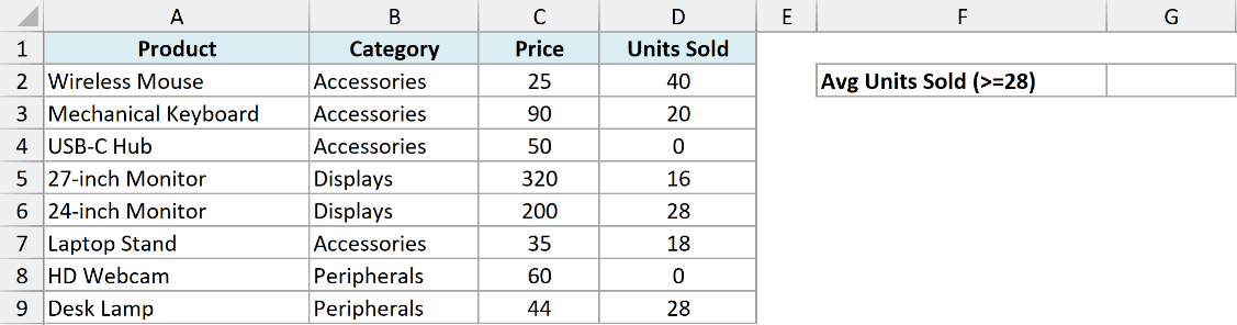
Here I want to average the same column I’m testing, so I don’t need the third argument at all.
Here is the formula:
=AVERAGEIF(D2:D9,">=28")
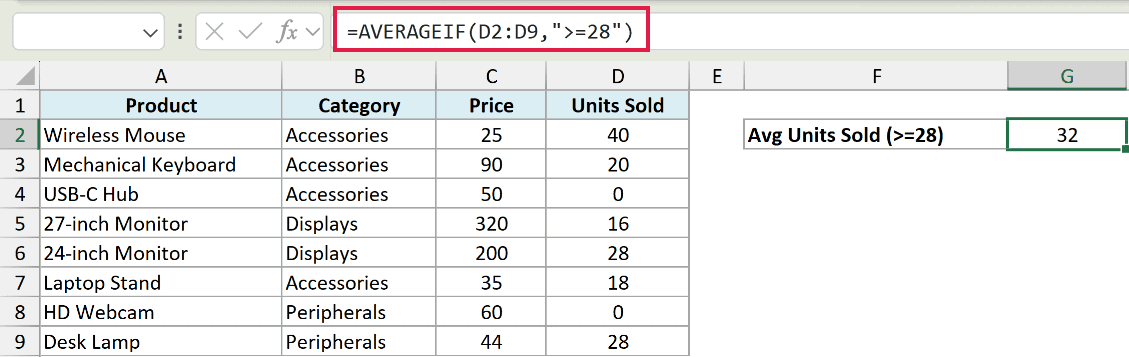
This returns 32.
Because I left out average_range, Excel checks each value in D2:D9 against the “>=28” condition and averages the ones that pass. Only three values clear the bar (40, 28, and 28), so the average is 32.
The comparison operator and the number both sit inside one set of quotes: “>=28”. You can use “>”, “<“, “>=”, “<=”, or “<>” the same way.
Example 3: Use a Cell Reference as the Criteria
Now let’s make the condition flexible instead of typing it into the formula.
Same product table as before. I’ve put the category I want in cell F2, and I want the average price for whatever category F2 holds. Right now F2 says Peripherals.
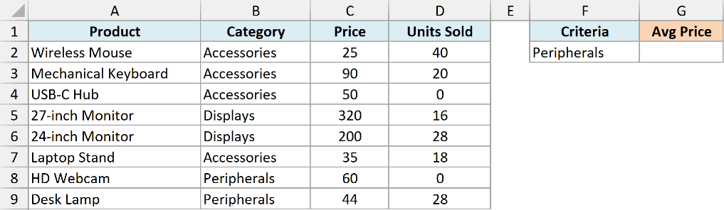
I want the average price of the category named in F2, so I can change the result just by changing that one cell.
Here is the formula:
=AVERAGEIF(B2:B9,F2,C2:C9)
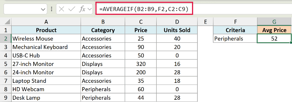
This returns 52.
Instead of hard-coding “Peripherals”, the criteria points to F2. Type a different category in F2 and the average updates on its own, which is handy for a small dashboard.
Pro Tip: To use an operator with a cell reference, join them with an ampersand. For example, “>=”&F2 checks for values greater than or equal to whatever number sits in F2. The operator goes in quotes, the cell reference stays outside.
Example 4: Average Using a Wildcard Criteria
Let’s look at partial-text matching, which is where wildcards come in.
Same product table. Say the products don’t have a tidy category I can rely on, but every monitor has the word “Monitor” in its name. I want the average price of all of them.
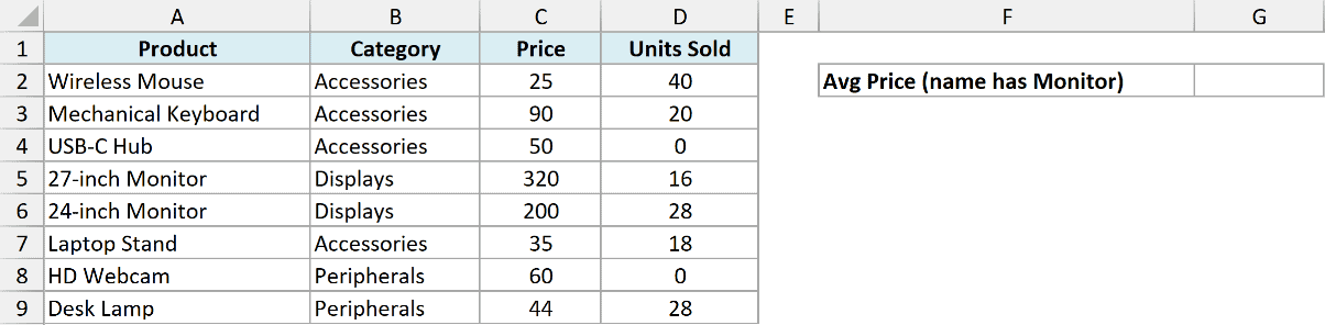
I want the average price of every product with “Monitor” anywhere in its name.
Here is the formula:
=AVERAGEIF(A2:A9,"*Monitor*",C2:C9)
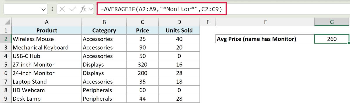
This returns 260.
The asterisks are wildcards. An asterisk (*) stands for any number of characters, so “*Monitor*” matches any name with “Monitor” in it, no matter what comes before or after.
You can also use a question mark (?) to stand for a single character. If you ever need to match a literal asterisk or question mark, put a tilde (~) in front of it.
Example 5: Average a Range and Ignore the Zeros
This one solves a problem that trips people up all the time.
Same product table. A couple of products were out of stock, so their units-sold value is 0. If I run a plain AVERAGE on the column, those zeros drag the result down. I want the average units sold across only the products that actually sold.
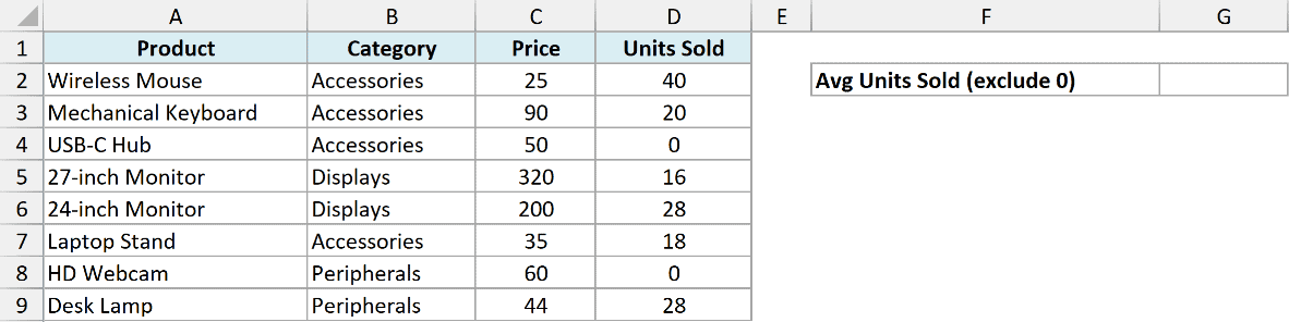
I want the average of the units-sold column, but with the zeros left out.
Here is the formula:
=AVERAGEIF(D2:D9,"<>0")
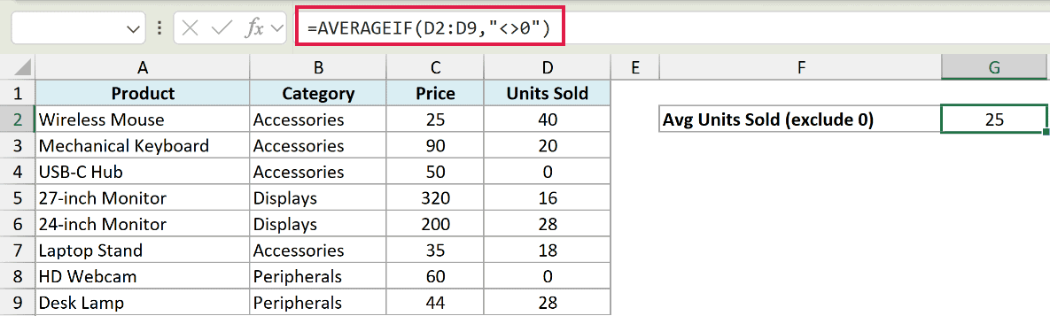
This returns 25.
The “<>” operator means “not equal to”, so “<>0” tells Excel to average every value except the zeros. Six products have non-zero sales, and their average is 25.
This matters because AVERAGEIF (like AVERAGE) counts zeros as real numbers. It only skips truly empty cells. So if a zero should not count as a data point, you have to exclude it yourself with “<>0”.
Example 6: Average One Column Based on Another
Let’s finish with the full three-argument form, where the condition lives in one column and the numbers you average live in another.
Same product table. I want the average units sold for the products priced above 50. So the condition sits in the price column, but the numbers I’m averaging are in the units-sold column.
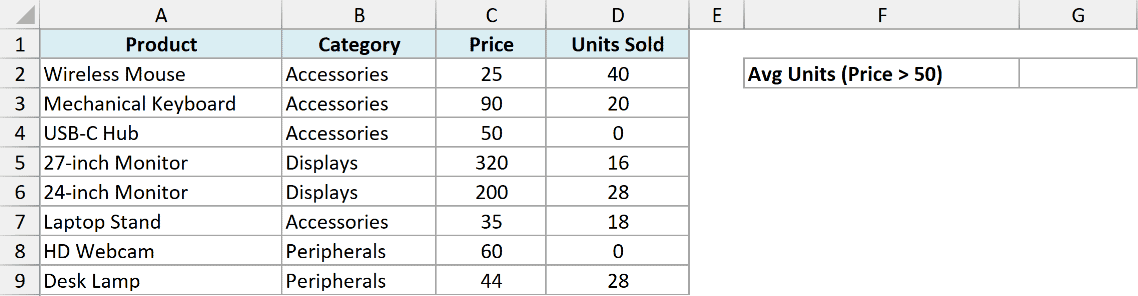
I want the average units sold for every product with a price above 50.
Here is the formula:
=AVERAGEIF(C2:C9,">50",D2:D9)
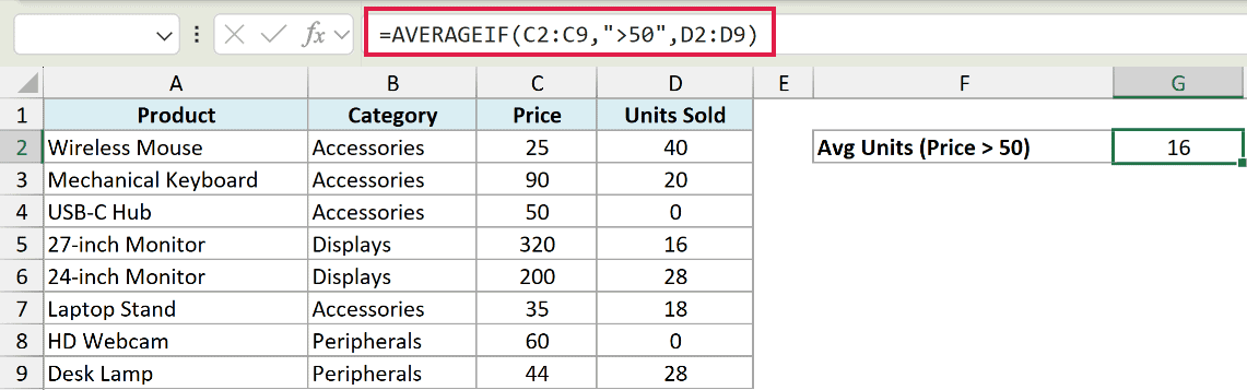
This returns 16.
Here the range (C2:C9) is the price column that gets checked against “>50”, and average_range (D2:D9) is the units-sold column that actually gets averaged. Four products cost more than 50, and the average of their units sold is 16.
Keep the range and average_range the same size and shape. Excel lines up average_range starting from its top-left cell, so a mismatched size can quietly average the wrong cells.
Tips & Common Mistakes
- A #DIV/0! error means nothing matched. If no cell in the range meets your criteria, there’s nothing to average and AVERAGEIF returns #DIV/0!. You’ll also see it if the cells you’re averaging are all empty or text. Here’s how to handle the #DIV/0! error if you want a clean result instead.
- Zeros are counted, blanks are not. AVERAGEIF treats a 0 as a real value but ignores truly empty cells. If zeros should not count, exclude them with “<>0” as in Example 5.
- Operators and text always need quotes. Conditions like “>100”, “<>0”, or “Accessories” go in double quotes. To combine an operator with a cell reference, join them with an ampersand, like “>=”&F2.
- One condition only. AVERAGEIF checks a single criteria. For two or more conditions at once, switch to the AVERAGEIFS function.
- It works with spilled ranges too. Since AVERAGEIF reads a whole range, you can feed it a spill reference from a dynamic array (in Excel 365 or 2021), like =AVERAGEIF(A2#,”>100″), and it averages the entire spilled result.
That covers the main ways to use AVERAGEIF in Excel. You’ve seen it average by a text category, by a numeric comparison, with wildcards, from a cell reference, while ignoring zeros, and across two different columns.
The same one-condition idea powers a whole family of functions. If you want a total instead of an average, SUMIF works the exact same way, and COUNTIFS does it for counting. And if you’d rather have the middle value than the average, there’s a MEDIAN IF trick too.
Once you’re comfortable with a single condition, AVERAGEIFS is the natural next step for averaging against several conditions at the same time.
Other Excel Articles You May Also Like:
