LOOKUP Function in Excel

If you want to find a value in a sorted row or column and pull back the matching item next to it, the LOOKUP function does exactly that.

It hunts for your value, and when there’s no exact hit, it settles on the largest value that isn’t bigger than what you asked for.

In Excel 365, you can also hand LOOKUP a whole range of lookup values and the answers spill into the cells below.

In this article, I’ll show you how to use LOOKUP with practical examples, covering both its vector and array forms.

LOOKUP Syntax

LOOKUP comes in two forms. Here is the vector form, which is the one you’ll use most:

=LOOKUP(lookup_value, lookup_vector, [result_vector])

• lookup_value – the value you want to find. This can be a number, text, a logical value, or a cell reference.
• lookup_vector – a single row or column, sorted in ascending order, that LOOKUP searches through.
• result_vector – optional. A single row or column holding the values you want returned. Leave it out and LOOKUP returns from lookup_vector itself.

LOOKUP has no exact-match-only switch. It returns an exact hit when there is one, otherwise the largest value less than or equal to your lookup value.

That makes it a quick way to find the closest match in a sorted list. For exact matching on unsorted data, use XLOOKUP instead.

Make sure result_vector has the same number of cells as lookup_vector. Absolute references stop one range from drifting when you copy the formula.

Also note that LOOKUP is case-insensitive. It can’t tell apart codes that differ only by letter case, so “AB10” and “ab10” look identical to it.

And here is the array form, which packs the search values and return values into one range:

=LOOKUP(lookup_value, array)

• array – a block of cells. If it’s wider than it is tall, LOOKUP searches the first row and returns from the last row. If it’s square or taller than wide, it searches the first column and returns from the last column.

LOOKUP works in Excel for Microsoft 365, Excel 2024, 2021, 2019, and 2016, plus Excel on the web. It’s a longstanding function, so you’ll find it in older workbooks too.

You can also check Microsoft’s LOOKUP function reference for the official argument rules.

When to Use the LOOKUP Function

Use LOOKUP when you need to:

• Map one or many values to bands in a small lookup vector that’s sorted in ascending order.
• Pull an as-of value from a vertical column pair or a horizontal row pair, where approximate matching is what you actually want.
• Keep older workbooks running, including the legacy array form and the classic last-value trick.
• Grab the final non-blank entry or the last matching record with the LOOKUP(2,1/(condition),result) pattern when backward compatibility matters.

LOOKUP vs VLOOKUP vs XLOOKUP

All three find a value and return something related to it, but they don’t behave the same way. Here’s a quick comparison:

	LOOKUP	VLOOKUP	XLOOKUP
Match type	Approximate only (exact when it finds one)	Exact or approximate	Exact by default, approximate optional
Needs sorted data	Yes, ascending	Only for approximate match	No
Where it returns from	Any row or column you point to	Only columns to the right	Any row or column you point to
When nothing matches	#N/A	#N/A	Your own message or value
Search from the bottom	Only with the 2,1/ trick	No	Yes
Available in	All versions	All versions	Excel 365, 2021 and later

LOOKUP is short and works in every version, but it quietly assumes your data is sorted.

For new work, I’d go with XLOOKUP when your Excel version and the people you share files with allow it.

When the file has to open in older Excel, VLOOKUP or HLOOKUP is the safer pick.

This breakdown of the difference between VLOOKUP and XLOOKUP covers that pair in detail.

Let me show you a few practical examples of how LOOKUP works.

Example 1: Assign Grades to Multiple Scores at Once

Let’s start with a spilling example, since that’s how you’ll most likely use LOOKUP in Excel 365.

Below is a simple grading table. The ascending score thresholds sit in A2:A6, with the matching grade in B2:B6. In E2:E7, I have the scores of six students.

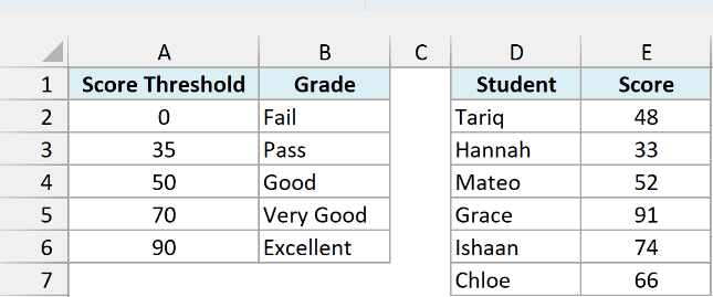
I want the right grade for every single student, all from one formula.

Here is the formula:

=LOOKUP(E2:E7,$A$2:$A$6,$B$2:$B$6)

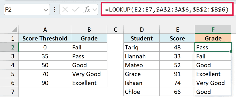
Because I fed LOOKUP the whole range E2:E7, it returns six answers that spill down the cells below. You type it once and Excel fills the rest.

For each score, LOOKUP finds the largest threshold that doesn’t go over it.

Tariq’s 48 lands on the 35 threshold and returns “Pass”, while Hannah’s 33 falls back to the 0 row and returns “Fail”.

Important: Sort the searched column in ascending order. If it isn’t sorted, LOOKUP can hand you a believable but wrong answer, with no error to warn you.

Also, if a score were smaller than the smallest threshold, LOOKUP would return #N/A. That’s why the table starts at 0.

In your own data, only wrap LOOKUP in IFNA when a below-minimum fallback actually makes sense.

Pro Tip: The spilling form needs Excel 365, Excel 2021 or later, or Excel for the web. In Excel 2019 or earlier, put =LOOKUP(E2,$A$2:$A$6,$B$2:$B$6) in F2 and copy it down.

Example 2: Look Up a Value Across a Row

Here’s another scenario, this time with data running sideways.

A gym revises its monthly fee every few months. The dates when each new fee started run across B1:G1, with the fee sitting right below in B2:G2.

In B5:B9, I have the join dates of five members.

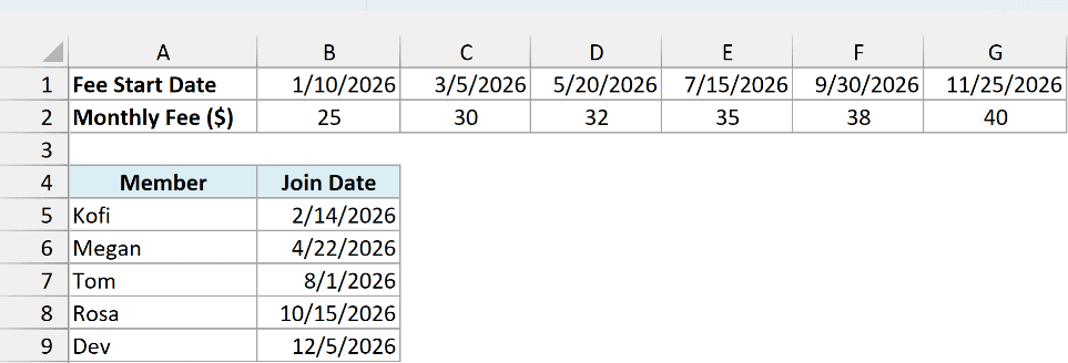
I want the fee that was active on each member’s join date, pulled from those horizontal rows.

Here is the formula:

=LOOKUP(B5:B9,$B$1:$G$1,$B$2:$G$2)

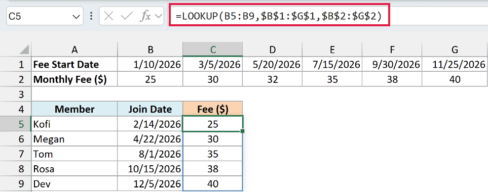
LOOKUP searches the start dates in B1:G1 for each join date, then returns the fee from the matching spot in B2:G2.

Tom joined on August 1, 2026. That lands on the July 15, 2026 revision, so he gets a fee of 35.

Notice that the source rows run horizontally, but the results still spill down a vertical list. The orientation of your lookup values decides the spill direction.

In Excel 2019 or earlier, enter =LOOKUP(B5,$B$1:$G$1,$B$2:$G$2) in C5 and copy it down instead.

Example 3: Use the Array Form of LOOKUP

Now let’s look at the array form, which handles the search and the return in a single range.

Below is a bulk-order discount table. Order quantities run in ascending order down column A, the delivery days sit in column B, and the discount is in column C.

The order quantity I want to check is in cell B9.

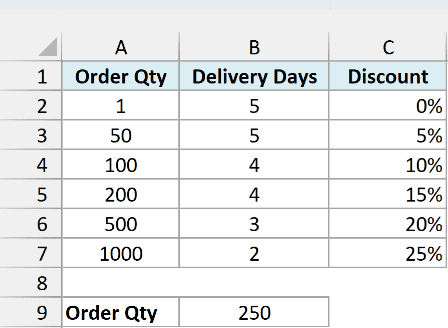
I want the discount for the quantity in B9, using the two-argument array form.

Here is the formula:

=LOOKUP(B9,A2:C7)

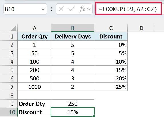
The range A2:C7 is taller than it is wide, so LOOKUP searches down the first column and returns from the last column.

An order of 250 lands on the 200 row and returns 15%.

The middle column, delivery days, is completely ignored.

The array form only ever uses the first and last columns of a tall range, so anything in between is just along for the ride.

Pro Tip: Microsoft keeps the array form mainly for old workbooks. For a new file, XLOOKUP is clearer, since you name the search and return columns directly.

Example 4: Get the Last Value in a Column

This next one is a handy trick for logs that keep growing.

I have a simple weight tracker with dates in column B and daily weights in C2:C11. It’s filled in through Day 7, and the rows below are still blank, waiting for future days.

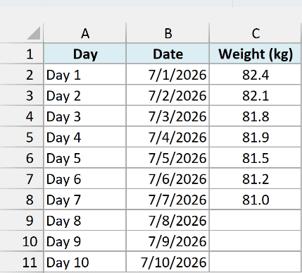
I want the last weight that’s actually been recorded, without hunting down the bottom row by hand every time.

Here is the formula:

=LOOKUP(2,1/(C2:C11<>""),C2:C11)

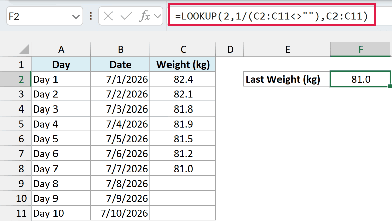
How this formula works:

• C2:C11<>”” checks each cell for content and builds an array of TRUE and FALSE values.
• 1/(…) turns every TRUE into 1 and every FALSE into a #DIV/0! error.
• LOOKUP(2, …) searches that array for 2. Since 2 is never found and LOOKUP skips the errors, it settles on the last 1, which is the final cell that has a value.
• LOOKUP then returns the weight from C2:C11 in that same position, which gives you 81.0.

Notice this returns a single value, not a spill. The condition builds an array internally, but LOOKUP still hands back only that one last item.

Point this formula at a real range like C2:C11 rather than a whole column, so it doesn’t calculate more cells than it needs to.

If your list holds only numbers, here’s another way to get the last number in a list.

Example 5: Find the Last Matching Record

Let’s build on that trick to pull the most recent record for one specific person.

I have a library loan log. The loan dates are in column A, member names in B2:B13, and the book borrowed in C2:C13. The member I want to check is in cell E2.

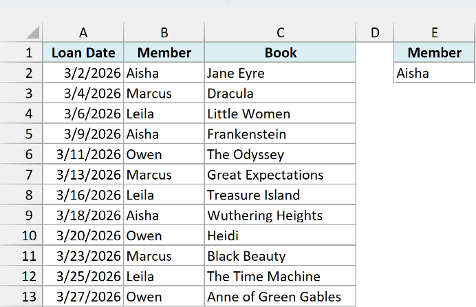
The same member shows up several times in the log, and I want the last book they borrowed.

Here is the formula:

=LOOKUP(2,1/(B2:B13=E2),C2:C13)

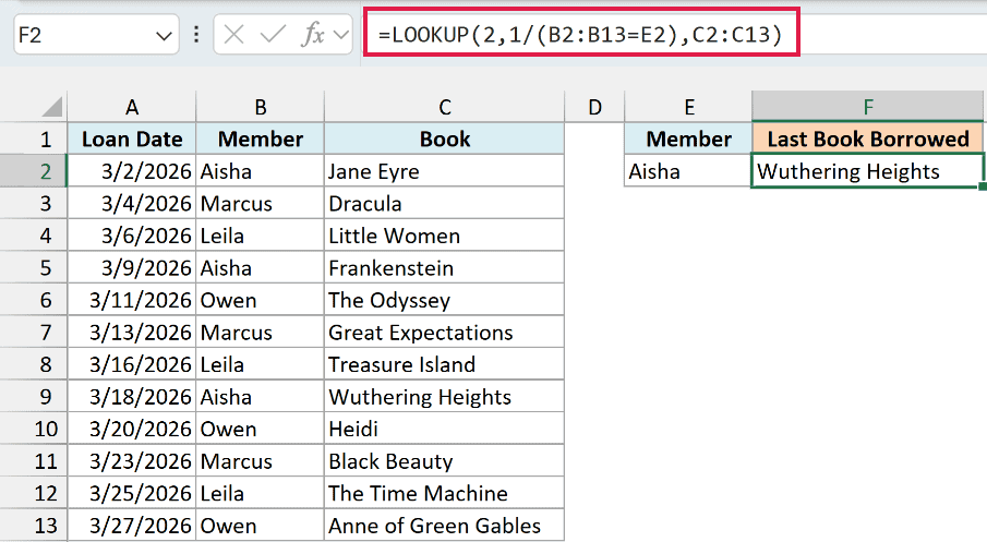
The condition B2:B13=E2 marks every row for Aisha as TRUE. Dividing 1 by that gives a 1 for each matching row and a #DIV/0! everywhere else.

LOOKUP hunts for 2, never finds it, and lands on the last 1, which is Aisha’s final loan. It then returns the book from C2:C13 in that spot, Wuthering Heights.

The same idea, tweaked a little, also lets you lookup the second or Nth value when you need something other than the last match.

I’ve also covered a few other ways to find the last occurrence of a lookup value, including a MAX-based formula and a VBA option.

Pro Tip: In Excel 365 or 2021, =XLOOKUP(E2,B2:B13,C2:C13,,0,-1) does the same job. The -1 tells XLOOKUP to search from the bottom up.

Example 6: Match on Two Conditions

Let’s finish with a tougher case: matching on more than one condition.

I have a grocery price log. The store is in B2:B13, the item in C2:C13, and the price paid in D2:D13. The store and item I care about are in G2 and G3.

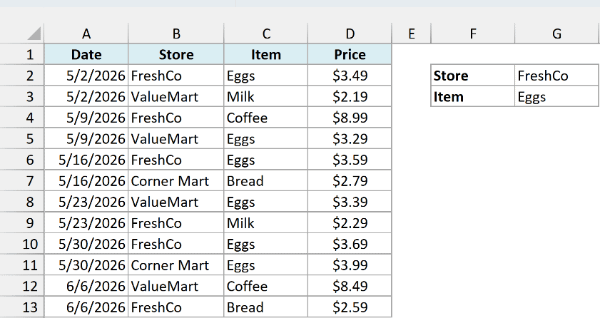
I want the latest price for the row that matches both the selected store and the selected item.

Here is the formula:

=LOOKUP(2,1/((B2:B13=G2)*(C2:C13=G3)),D2:D13)

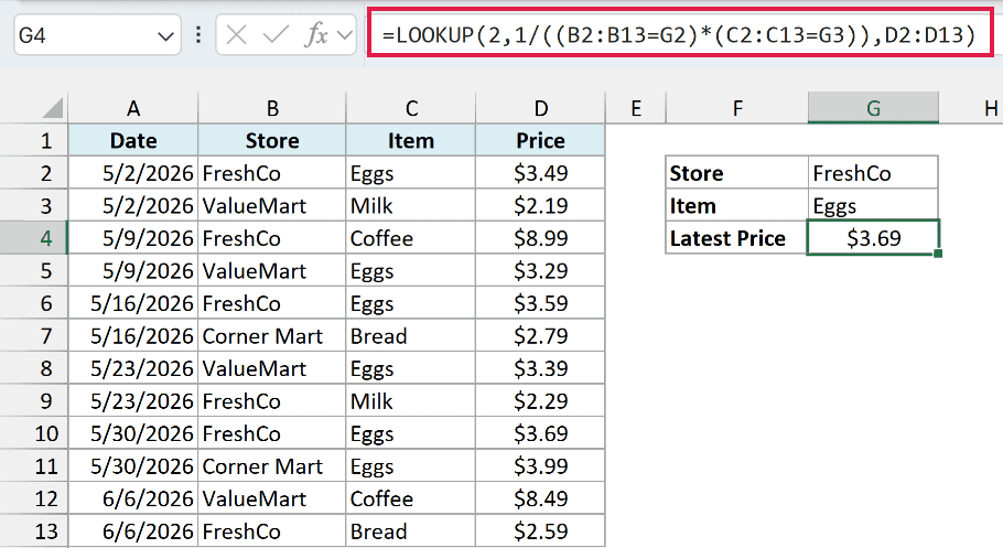
How this formula works:

• (B2:B13=G2) and (C2:C13=G3) each build a TRUE/FALSE array, one for the store and one for the item.
• Multiplying them gives 1 only where both are TRUE, since TRUE times TRUE is 1 and anything with a FALSE becomes 0.
• 1/(…) turns those 1s into 1 and the 0s into #DIV/0! errors.
• LOOKUP(2, …) settles on the last 1, so you get the price from the most recent row that matches both conditions.

Here that’s $3.69, from the May 30 FreshCo eggs row. It skips the later Corner Mart eggs and FreshCo bread rows, since each of those matches only one condition.

Keep in mind this returns one value, the latest match. If you want every matching row instead, FILTER is the cleaner route in Excel 365.

And for just the latest match in Excel 365 or 2021, =XLOOKUP(1,(B2:B13=G2)*(C2:C13=G3),D2:D13,,0,-1) reads more plainly.

If you’re working with VLOOKUP, here’s how to use VLOOKUP with multiple criteria.

LOOKUP is a handy way to match a value against a sorted list and pull back the item beside it, whether your data runs down a column or across a row.

It’s still worth knowing, both for older files and for those compact last-match and approximate-match jobs.

I hope you found this tutorial helpful.

List of All Excel Functions

Other Excel Articles You May Also Like:

• VLOOKUP Function in Excel (10 Examples)
• HLOOKUP Function in Excel (4 Examples)
• INDEX & MATCH Functions Combo in Excel (10 Easy Examples)