UNIQUE Function in Excel

If you want a clean list of distinct values from a column full of repeats, the UNIQUE function is what you’re looking for.

You point it at a range and it hands back one of each value. You don’t need the Remove Duplicates dialog, and your original data stays untouched.

UNIQUE is a dynamic array function. It spills its results into the cells below, and the list updates on its own when the source values change.

In this article, I’ll show you how UNIQUE works with 8 practical examples, from a plain distinct list to a drop-down that grows with your data.

Excel UNIQUE Function Syntax

Here is the syntax of the UNIQUE function:

=UNIQUE(array, [by_col], [exactly_once])

• array – the range or array you want the distinct values from. This is the only required argument.
• by_col – optional. Leave it out (or use FALSE) and UNIQUE compares rows. Use TRUE when your data runs across a row and you want to compare columns instead.
• exactly_once – optional. Leave it out (or use FALSE) and you get one of every distinct value. Use TRUE and you get only the values that appear a single time.

So =UNIQUE(B2:B13) on its own compares rows and returns one of each value, in the order each one first appears.

The two optional arguments are positional. To set exactly_once without by_col, leave an empty slot with an extra comma, like =UNIQUE(B2:B13,,TRUE).

UNIQUE is also non-volatile. It only recalculates when the data it points to changes, so it won’t slow your workbook down.

Important: UNIQUE works in Microsoft 365, Excel 2024, and Excel 2021 (Windows and Mac), and in Excel for the web. Excel 2019 and earlier don’t have it and show a #NAME? error.

If you’re on one of those older versions, you can get a unique list with the Remove Duplicates or Advanced Filter options on the Data tab.

When to Use the UNIQUE Function

Use UNIQUE when you need to:

• Pull one of each value from a column without touching the original data.
• Find the values that appear only once, like customers who ordered a single time.
• Get the distinct combinations across two or more columns.
• Build a sorted, blank-free list that refreshes itself when the data changes.
• Feed a live list into a count, a drop-down, or a small formula-driven report.

Let me show you a few practical examples of how UNIQUE works.

Example 1: Get Unique Values from a Column

Let’s start with the simplest case, which is also the one you’ll use most.

Below is an order log. Each row is one order, and column B has the product that was ordered. The same products keep coming up in B2:B13.

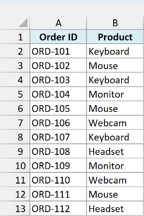
I want a list of every product that has been ordered, with each product shown only once.

Here is the formula:

=UNIQUE(B2:B13)

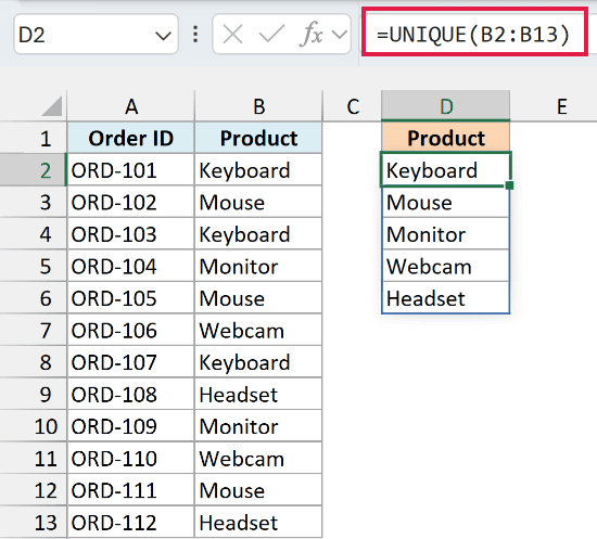
This returns five products: Keyboard, Mouse, Monitor, Webcam, and Headset. You enter the formula once in D2 and the whole list spills down.

Notice the order. UNIQUE keeps each value where it first shows up in the source, so Keyboard comes first because it’s the first product in column B.

It doesn’t sort anything. Example 2 shows how to get the list in A-to-Z order.

Important: The cells where the result spills (D2:D6 here) must be empty. If anything is in the way, you get a #SPILL! error until you clear those cells.

Pro Tip: A fixed range like B2:B13 won’t pick up new rows you add below it. This is true for every example in this article. Example 8 shows how an Excel Table fixes this.

Example 2: Sort Unique Values and Ignore Blanks

Here’s a common wrinkle. Real columns have gaps, and UNIQUE treats a blank cell as a value too, so it shows up in the result as a 0.

Let’s clean that up and sort the list while we’re at it.

Below is a shipment log. Column B has the destination city for each shipment, and two rows (B4 and B9) were never filled in.

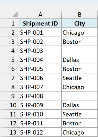
I want an A-to-Z list of the cities, with no blank item in it.

Here is the formula:

=SORT(UNIQUE(FILTER(B2:B13,B2:B13<>"")))

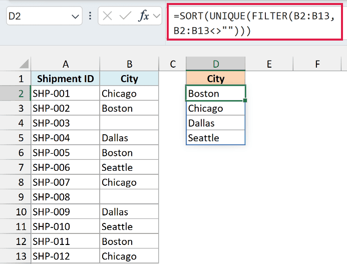
This returns a sorted list: Boston, Chicago, Dallas, and Seattle.

How this formula works:

• FILTER(B2:B13,B2:B13<>””) keeps only the cells that aren’t blank, so the empty rows never reach UNIQUE.
• UNIQUE takes that blank-free list and returns one of each city.
• SORT puts the cities in A-to-Z order.

It’s still one formula that spills, and it re-sorts itself the moment a new city shows up in column B.

Important: UNIQUE ignores case, so ACME and Acme count as one value. But “Boston ” with a trailing space counts as a separate city. Clean such data with TRIM first.

Example 3: Find Values That Appear Exactly Once

This is where the third argument comes in. By default, UNIQUE gives you one of every value.

Set exactly_once to TRUE and it keeps only the values that never repeat. Anything that shows up more than once is dropped completely.

Below is a gym check-in log. Column B has the member name for each visit. Most members came in more than once, but a few came in just once.

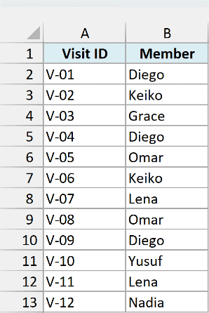
I want just the members who checked in exactly once, so I can see who never came back for a second visit.

Here is the formula:

=UNIQUE(B2:B13,,TRUE)

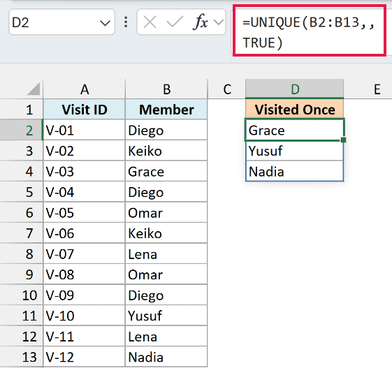
This returns the three members who appear a single time: Grace, Yusuf, and Nadia. Diego, Keiko, Omar, and Lena all came back, so none of them show up.

Note the double comma. I’m leaving by_col at its default, so I skip it with an empty slot and put TRUE in the third position.

Important: Use TRUE only when you want values that appear once. For one of each value, leave it out. Also, if every value repeats, you get a #CALC! error.

Example 4: Get Unique Rows Across Multiple Columns

UNIQUE isn’t limited to a single column. Give it a two-column range and it compares whole rows, returning each distinct combination.

Below is an expense log. Column B has the department, column C has the expense type, and the same pairs repeat across B2:C13.

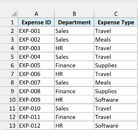
I want each distinct department and expense type combination, listed once.

Here is the formula:

=UNIQUE(B2:C13)

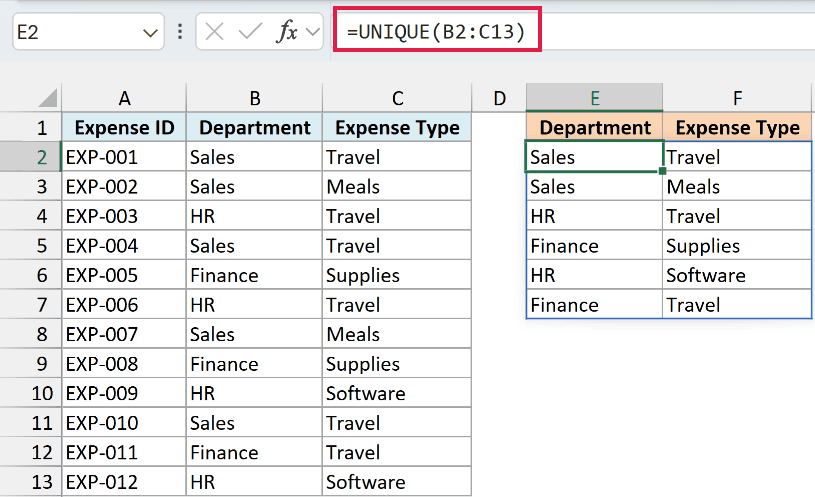
This spills six rows across two columns. Each row is one distinct pair, like Sales + Travel, Sales + Meals, and HR + Travel.

Notice that “Travel” repeats in the result. That’s fine, because Sales + Travel and HR + Travel are different rows. UNIQUE looks at the full row, not each column by itself.

Example 5: Get Unique Values Across a Row (by_col)

So far the data has run down a column. When your data runs across a row instead, that’s where the by_col argument comes in.

Below is a cafeteria menu plan laid out sideways. The special dish for each month sits in B2:M2, and the same dishes repeat across the year.

I want the distinct dishes served across the year, and I want the result to stay horizontal.

Here is the formula:

=UNIQUE(B2:M2,TRUE)

This returns Pasta, Tacos, Curry, and Burgers, and the result spills to the right from B4.

Setting by_col to TRUE tells UNIQUE to compare columns instead of rows. Leave it out here and UNIQUE sees one single row, so it hands the whole row back unchanged.

Example 6: Extract Unique Values Based on Criteria

Often you don’t want every distinct value, only the ones that meet a condition. The FILTER function handles the condition and UNIQUE removes the repeats.

Below is a customer complaint log. Column B has the store each complaint came from, and column C has its priority.

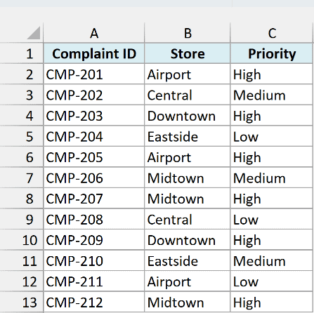
I want an A-to-Z list of the stores that logged at least one High-priority complaint.

Here is the formula:

=SORT(UNIQUE(FILTER(B2:B13,C2:C13="High")))

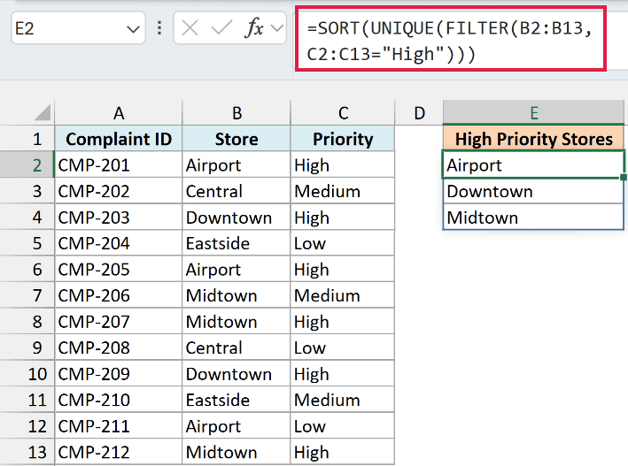
This returns Airport, Downtown, and Midtown.

How this formula works:

• FILTER(B2:B13,C2:C13=”High”) returns the store names from rows where the priority is High.
• UNIQUE reduces that to one of each store, since Airport, Downtown, and Midtown each logged more than one High complaint.
• SORT puts the stores in A-to-Z order.

You don’t need a helper column or a pivot table. Change a priority in column C to High and the store list updates on its own.

Pro Tip: If no row matches, FILTER returns a #CALC! error. To show a message instead, use its third argument, like FILTER(B2:B13,C2:C13=”High”,”None”).

Example 7: Count Unique Values That Match a Condition

You can also use UNIQUE as an ingredient rather than the final answer. Wrap it in ROWS and you get a count of the distinct values instead of the list.

Below is a movie ticket log. Column B has the movie, column C has the showtime, and the showtime I want to check is in cell F1.

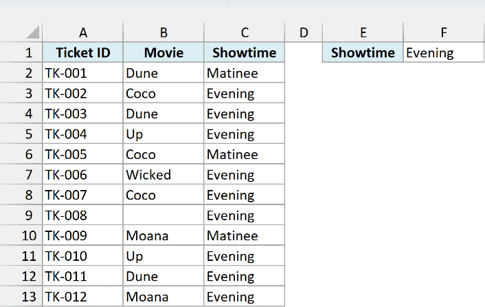
I want to count how many different movies played in the showtime in F1 (Evening), skipping the ticket where the movie is blank.

Here is the formula:

=ROWS(UNIQUE(FILTER(B2:B13,(C2:C13=F1)*(B2:B13<>""))))

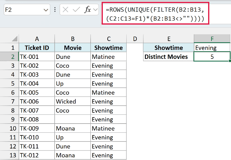
This returns 5, because Coco, Dune, Up, Wicked, and Moana all played in the Evening slot.

How this formula works:

• FILTER keeps the movie names where the showtime matches F1 and the movie cell isn’t blank. The two conditions are multiplied, so both have to be true.
• UNIQUE reduces those movies to the distinct ones.
• ROWS counts how many rows that distinct list has, which is your answer.

Without the blank check, the empty movie cell on TK-008 would count as one more distinct value, and you’d get 6.

Important: If nothing matches, this formula returns #CALC! instead of 0. Wrap it as IFERROR(ROWS(…),0). A FILTER fallback like “” would wrongly count 1.

If you’re on Excel 2019 or earlier, see my guide on how to count unique values in Excel with COUNTIF.

Example 8: Create a Drop-Down List of Unique Values

A UNIQUE list makes a great source for a drop-down list. When it’s fed by an Excel Table, the drop-down grows and shrinks as the data does.

Below is an Excel Table named TableBookings. Its Venue column has the training room for each booking, with repeats and two bookings where no venue was recorded yet.

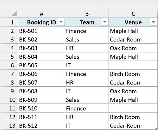
I want a sorted, blank-free list of venues, and then a drop-down in H1 that offers only those venues.

Here is the formula (entered in E2, outside the Table):

=SORT(UNIQUE(FILTER(TableBookings[Venue],TableBookings[Venue]<>"")))

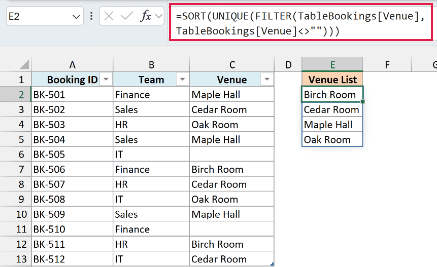
This returns Birch Room, Cedar Room, Maple Hall, and Oak Room. FILTER drops the blank venues, UNIQUE removes the repeats, and SORT keeps the list A-to-Z.

Because the formula refers to the Table column, any booking you add to the Table is picked up automatically. That’s the fix for the fixed-range problem from Example 1.

Important: Enter the formula outside the Table. A formula that spills can’t return results inside an Excel Table, so it shows a #SPILL! error there.

Now let’s use this list as the source of a drop-down. Here are the steps:

1. Select cell H1, where you want the drop-down.

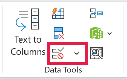
2. Go to the Data tab and click Data Validation.

3. In the Allow drop-down, select List, and in the Source box, enter =$E$2#. Then click OK.

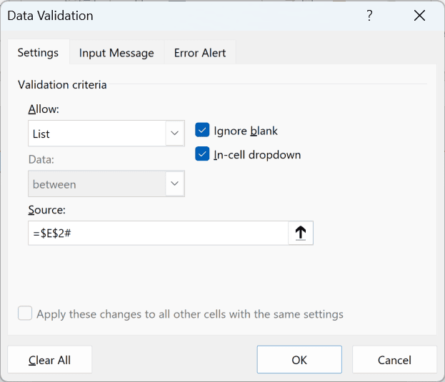
Now H1 has a drop-down with the four venues.

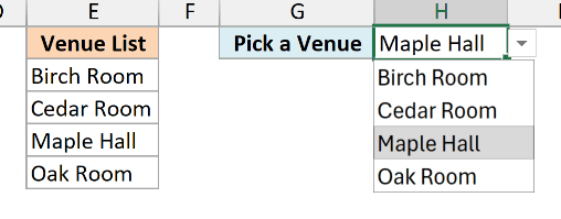
The # after E2 is the spill operator. It means “the entire spilled range that starts in E2”, so the drop-down always matches the current length of the list.

Add a booking with a new venue to the Table and it flows into the list and the drop-down, without touching the validation settings.

For more drop-down options, see my guide on creating a drop down list in Excel.

UNIQUE turns a column of repeats into a clean, live list with one formula. Pair it with SORT and FILTER for sorted or filtered lists, and with ROWS for a count.

I hope you found this tutorial helpful.

List of All Excel Functions

Other Excel Articles You May Also Like:

• Find and Remove Duplicates in Excel
• Creating Multiple Drop-down Lists in Excel without Repetition
• COUNTIFS Function in Excel
• SUMIF Function in Excel
• 20 Advanced Excel Functions and Formulas (for Excel Pros)
• Remove Blank Rows in Excel Using a Formula
• Remove Duplicates Within a Cell in Excel