

The INTERCEPT function in Excel finds the point where a straight best-fit line through your data crosses the y-axis. In plain terms, it tells you what y would be when x is zero.
That makes it handy for finding a fixed starting amount hidden in your data, like a base fee before any usage is added.
In this article, I’ll show you how to use INTERCEPT with six practical examples, including a couple of traps that give you a wrong number without any error.
Follow along with the example file
INTERCEPT Function Examples.xlsx
INTERCEPT Function Syntax
Here is the syntax of the INTERCEPT function:
=INTERCEPT(known_y's, known_x's)
- known_y’s – The values you want to explain or predict (the dependent values), like the fare paid for each taxi ride.
- known_x’s – The values that drive them (the independent values), like the miles traveled on each ride.
Both arguments are required, and the y values always come first. This is the opposite of how most people read a chart (x, then y), so it’s an easy one to mix up.
Both ranges need the same number of values. If one range has 10 cells and the other has 11, INTERCEPT returns the #N/A error.
INTERCEPT also needs at least two different x values to draw a line. If all your x values are the same (or you only have one data point), you get the #DIV/0! error.
The INTERCEPT function works in all Excel versions, including Microsoft 365, 2024, 2021, 2019, 2016, Mac, and the web.
When to Use the INTERCEPT Function
Use this function when you need to:
- Find a fixed fee or base cost hidden inside a list of prices, like a taxi’s starting fare
- Get the starting value of a trend, like a runner’s time before training began
- Write out the equation of a trendline (y = mx + b) together with the SLOPE function
- Compare the base amount for different groups in the same table
Let me show you a few practical examples of how to use INTERCEPT in Excel.
Example 1: Find the Y-Intercept in Excel (Base Taxi Fare)
Let’s start with a simple example.
Below I have a list of taxi rides with the miles traveled and the fare paid for each ride, and I want to find the base fare (what the meter charges before any miles) in cell E2.
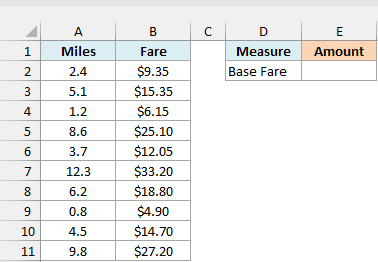
Here is the formula:
=INTERCEPT(B2:B11,A2:A11)
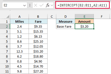
This gives us $3.20.
In the above formula, B2:B11 has the fares (the y values) and A2:A11 has the miles (the x values). INTERCEPT fits a straight line through these ten rides and returns the fare where that line sits at zero miles.
That’s the base fare. Every ride starts at about $3.20, and the per-mile charge gets added on top of it.
Important: If you swap the two ranges, INTERCEPT doesn’t show an error. It simply returns a different number (the miles you’d travel for a $0 fare), so always put the y values first.
Example 2: Get the Slope and Intercept of a Line
The intercept is only half of a straight line. The other half is the slope, and together they give you the full equation.
Below I have a plumber’s past jobs with the hours worked and the invoice amount, and I want the call-out fee, the hourly rate, and the line equation in column E.
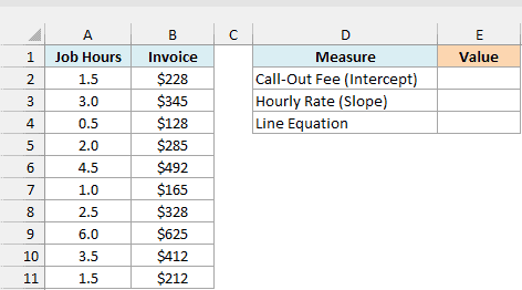
Here is the formula for the call-out fee in E2:
=INTERCEPT(B2:B11,A2:A11)
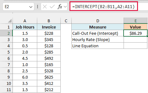
This returns $86.29, which is what the plumber charges just for showing up, before any hours are added.
Now here is the formula for the hourly rate in E3:
=SLOPE(B2:B11,A2:A11)
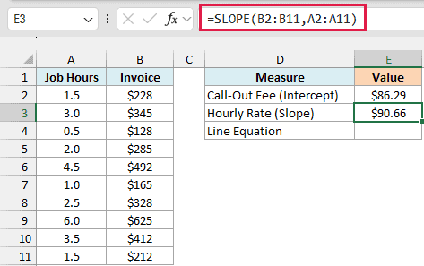
This returns $90.66. The SLOPE function takes the same two ranges in the same order, and it tells you how much the invoice goes up for each extra hour of work.
And here is the formula that puts both numbers into one equation in E4:
="y = "&TEXT(E3,"0.00")&"x + "&TEXT(E2,"0.00")
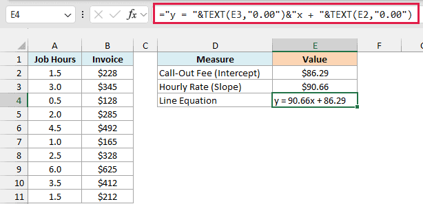
This shows y = 90.66x + 86.29. The TEXT function rounds each number to two decimals, and the & operator joins them with the rest of the equation text.
This is the same equation Excel shows when you add a linear trendline to a scatter chart of this data.
The plus sign is typed into the formula, so if your intercept is negative (like in the next example), you’ll see “+ -” in the result.
Pro Tip: To estimate the invoice for a new job, use the FORECAST.LINEAR function (Excel 2016 and later), like =FORECAST.LINEAR(5,B2:B11,A2:A11). It returns $539.58 for a 5-hour job, the same as E2 plus 5 times E3.
Example 3: When the Intercept Has No Real-World Meaning
The intercept doesn’t always mean something in real life. This example shows what that looks like.
Below I have a coffee cart’s daily sales with the temperature that day and the number of iced coffees sold, and I want to find the intercept (the cups sold at 0°F) in cell E2.
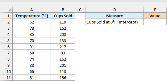
Here is the formula:
=INTERCEPT(B2:B11,A2:A11)
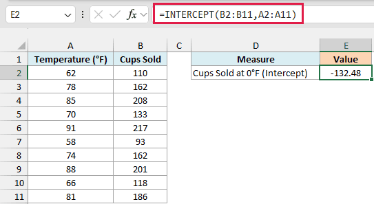
This returns -132.48.
The math is correct. The line through these ten days drops as it gets colder, and if you keep extending it all the way down to 0°F, it ends up at -132 cups sold.
Of course, nobody sells negative cups of coffee. The coldest day in this data is 58°F, so 0°F is far outside anything the line was built from.
So in this case, the intercept is just the spot where the line is anchored, and it isn’t a forecast for a freezing day. It’s still useful as part of the line equation, as we saw in Example 2.
As a rule of thumb, only read the intercept as a real value when x = 0 makes sense for your data. Zero miles in a taxi works, while 0°F for an iced coffee cart doesn’t.
Example 4: INTERCEPT With Missing Data
Real data often has gaps, and INTERCEPT handles those quietly.
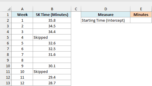
Below I have a 12-week 5K training log with a few weeks marked “Skipped” or left blank, and I want to find the estimated starting time (before week 1) in cell E2.
Here is the formula:
=INTERCEPT(B2:B13,A2:A13)
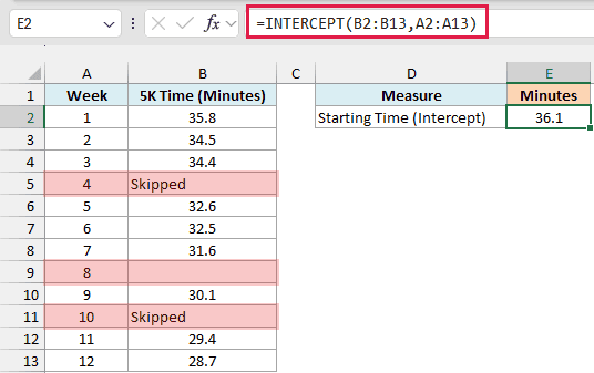
This returns 36.1 minutes, which is the runner’s estimated 5K time at week 0, before the training started.
When a cell in either range has text, a TRUE/FALSE value, or nothing at all, INTERCEPT skips that whole row. Here, weeks 4, 8, and 10 are left out, and the result comes from the nine weeks that have a time.
You don’t need to clean up the data first. Removing those three rows by hand would give you exactly the same 36.1.
Note that this only applies to text, TRUE/FALSE values, and blanks. If a cell has an error like #DIV/0! or #N/A, INTERCEPT returns that error instead of skipping it, so fix the errors before using the formula.
Example 5: Calculate the Intercept for Each Group (with FILTER)
INTERCEPT doesn’t have a built-in way to check a condition, but you can feed it filtered data instead.
Below I have a list of deliveries from three courier companies with the miles and the delivery fee, and I want to find the base fee for each courier in column F.
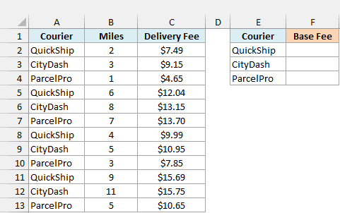
Here is the formula for F2, which I then copied down to F4:
=INTERCEPT(FILTER($C$2:$C$13,$A$2:$A$13=E2),FILTER($B$2:$B$13,$A$2:$A$13=E2))
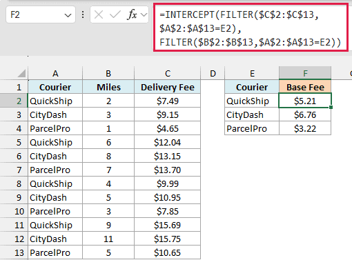
This gives a base fee of $5.21 for QuickShip, $6.76 for CityDash, and $3.22 for ParcelPro.
How this formula works:
- FILTER($C$2:$C$13,$A$2:$A$13=E2) pulls out only the fees for the courier named in E2. These become the y values.
- FILTER($B$2:$B$13,$A$2:$A$13=E2) pulls out the miles for the same courier, in the same order. These become the x values.
- INTERCEPT then fits a line through just those deliveries and returns that courier’s base fee.
The ranges are locked with dollar signs so they stay the same as you copy the formula down. Only E2 changes, to E3 and then E4.
If a courier name in column E doesn’t appear in the data, FILTER finds nothing and the formula returns the #CALC! error. So make sure the names match the ones in column A exactly.
The FILTER function is available in Excel for Microsoft 365, Excel 2021, and later. If you are using Excel 2019 or earlier, enter the below formula in cell F2 with Ctrl + Shift + Enter, and then copy it down to F4:
=INTERCEPT(IF($A$2:$A$13=E2,$C$2:$C$13,""),IF($A$2:$A$13=E2,$B$2:$B$13,""))
It returns the same three base fees. The IF function keeps the fee and the miles only for the matching courier and turns every other row into empty text, which INTERCEPT then skips.
Example 6: INTERCEPT With Dates
This last one is a trap, because the formula works but the answer makes no sense.
Below I have a sunflower’s height measured on different dates over seven weeks, and I want to find its estimated height on the first day in column E.
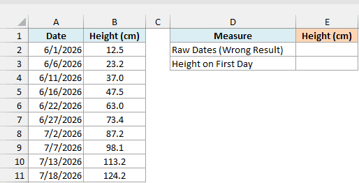
Here is the formula you’d probably try first, in E2:
=INTERCEPT(B2:B11,A2:A11)
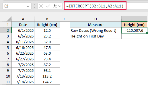
This returns -110,507.6 cm, which is clearly wrong for a sunflower.
Here’s why it happens. Excel stores dates as numbers counting from January 1, 1900, so 6/1/2026 is really 46174 behind the scenes.
So when INTERCEPT works out the value at x = 0, it’s estimating the plant’s height back in 1900. Running the line back that many days gives you a huge negative number.
To fix this, count the days from the first date instead. Here is the formula in E3:
=INTERCEPT(B2:B11,A2:A11-A2)
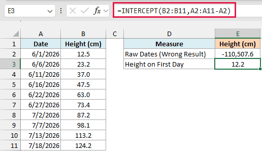
This returns 12.2 cm, which is the plant’s estimated height on 6/1/2026, the first day of measuring.
In the above formula, A2:A11-A2 subtracts the first date from every date, so the x values become 0, 5, 10, and so on. Now x = 0 is the first day, and the intercept is the height on that day.
This works because the dates are in order, so A2 is the earliest one. If your dates aren’t sorted, subtract MIN(A2:A11) instead of A2, so the earliest date becomes day 0.
You can also get the same 12.2 with =FORECAST.LINEAR(A2,B2:B11,A2:A11), which estimates the height on any date you give it.
So these are six practical ways to use the INTERCEPT function in Excel, from finding a simple base fare to working with groups and dates.
If your x values are dates, count the days from the first date before you use INTERCEPT, or you’ll get the value back in 1900.
Other Excel Articles You May Also Like:
