

The ERROR.TYPE function tells you which error a cell has. It returns a number for each error type, like 2 for #DIV/0! and 3 for #VALUE!, so a formula can react to one kind of error and leave the others alone.
Functions like IFERROR treat every error the same way. ERROR.TYPE is the one you reach for when a #DIV/0! needs a different fix than a typo in a lookup, and you want your sheet to say which is which.
In this article, I’ll show you the number for each error and how to turn those numbers into your own messages. I’ll also cover the one catch, which is that a cell with no error gets #N/A instead of a number.
Follow along with the example file
ERROR.TYPE Function Examples.xlsx
ERROR.TYPE Function Syntax
Here is the syntax of the ERROR.TYPE function:
=ERROR.TYPE(error_val)
- error_val – The value you want to check. This is usually a cell reference, but it can also be a calculation, a range of cells, or an error typed straight into the formula, such as #REF!.
When you give ERROR.TYPE a calculation, it runs the calculation first and then checks the answer. When you give it a range (in Excel 365 and 2021 or later), it returns one number for each cell, and the results spill into the cells below.
Here is the number ERROR.TYPE returns for each error:
| Error | Number |
|---|---|
| #NULL! | 1 |
| #DIV/0! | 2 |
| #VALUE! | 3 |
| #REF! | 4 |
| #NAME? | 5 |
| #NUM! | 6 |
| #N/A | 7 |
| #GETTING_DATA | 8 |
| #SPILL! | 9 |
| #CALC! | 14 |
If the value isn’t an error at all (a number, text, or a blank cell), ERROR.TYPE returns #N/A. The #SPILL! and #CALC! errors only exist in Excel 365 and 2021 or later, so you’ll only see 9 and 14 there.
The ERROR.TYPE function works in all Excel versions, including 365, 2024, 2021, 2019, 2016, and Mac.
When to Use the ERROR.TYPE Function
Use this function when you need to:
- Find out which error each cell in a column has, not just that it has one.
- Check a calculation for errors before you add a column for it.
- Show a different message for each kind of error.
- Pull out the rows that have one specific error so you can fix them.
- Tell apart the newer dynamic array errors, like #SPILL! and #CALC!.
Let me show you a few practical examples of how to use this function.
Example 1: Get the Error Code for Each Cell
Let’s start with a simple example.
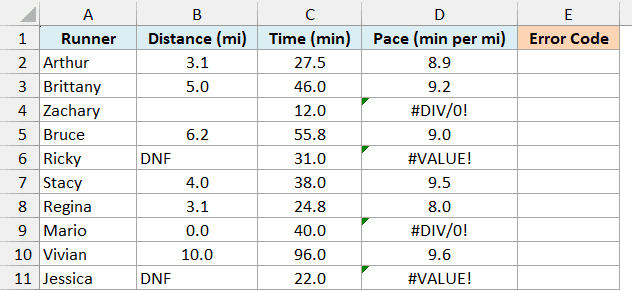
Below is a running log with each runner’s distance and time, where the pace column has a few errors, and I want to get the error code for each pace in column E.
Here is the formula:
=ERROR.TYPE(D2:D11)
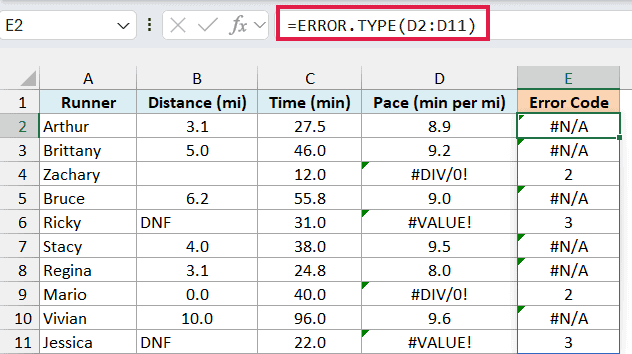
You enter this formula once in cell E2, and in Excel 365 and 2021 or later the results spill down to E11. ERROR.TYPE checks each pace in D2:D11 and returns the number for every cell that has an error.
Zachary and Mario get 2, because a blank or 0 distance makes the pace a #DIV/0! error. Ricky and Jessica get 3, because their distance is the text “DNF”, and dividing by text gives #VALUE!.
Important: The #N/A in the other rows doesn’t mean those paces have an error. It’s how ERROR.TYPE says “no error here”, and a real #N/A error would return 7 instead.
The same goes for text that only looks like an error. If a cell holds the text “#N/A” (which can happen with imported data), ERROR.TYPE returns #N/A for it, because it isn’t a real error.
If you are using Excel 2019 or earlier, enter the below formula in cell E2 and then copy it down the range:
=ERROR.TYPE(D2)
Example 2: Show a Blank When There’s No Error
That #N/A for rows without an error makes the results hard to scan. Here’s how to hide it.
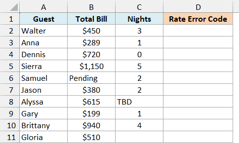
Below is a list of hotel bookings with the total bill and the number of nights, and before I work out the nightly rate, I want to see which rows would give an error in column D.
Here is the formula:
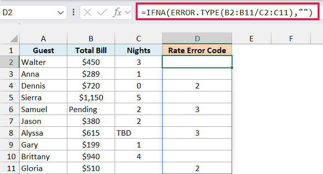
=IFNA(ERROR.TYPE(B2:B11/C2:C11),"")
How this formula works:
- B2:B11/C2:C11 divides each total bill by its nights right inside the formula, so you don’t need a nightly rate column to check it.
- ERROR.TYPE returns the error number for each division that fails, and #N/A for the ones that work.
- The IFNA function replaces each #N/A with an empty string (“”), so the rows without an error stay blank.
Dennis and Gloria get 2, because their nights are 0 and blank, which gives #DIV/0!. Samuel gets 3 because his bill says “Pending”, and Alyssa gets 3 because her nights say “TBD”.
The IFNA function is safe here because it can’t hide a real error. A division that really returned #N/A would get the number 7 from ERROR.TYPE, so only the “no error” #N/A gets replaced.
If you are using Excel 2019 or 2016, enter the below formula in cell D2 and then copy it down the range:
=IFNA(ERROR.TYPE(B2/C2),"")
Example 3: Show a Custom Message for Each Error Type
Now let’s look at something more useful, where each error gets its own plain-English message.
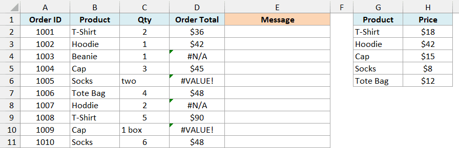
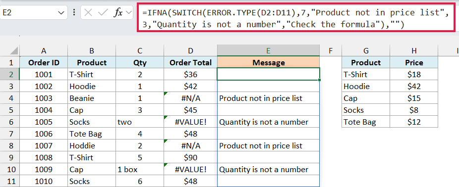
Below is a list of T-shirt store orders, where the order total looks up each product’s price and multiplies it by the quantity, and I want to show what went wrong with each error in column E.
Here is the formula:
=IFNA(SWITCH(ERROR.TYPE(D2:D11),7,"Product not in price list",3,"Quantity is not a number","Check the formula"),"")
How this formula works:
- ERROR.TYPE(D2:D11) returns 7 for each #N/A, 3 for each #VALUE!, and #N/A for the orders without an error.
- The SWITCH function compares each number with the ones you list. A 7 becomes “Product not in price list”, a 3 becomes “Quantity is not a number”, and any other error number gets the last value, “Check the formula”.
- The IFNA function turns the #N/A from the orders without an error into a blank.
Orders 1003 and 1007 get the price list message, because “Beanie” isn’t in the list and “Hoddie” is a typo. Orders 1005 and 1009 get the quantity message, because “two” and “1 box” are text.
You’ll often see ERROR.TYPE paired with the CHOOSE function for this, since Microsoft’s own ERROR.TYPE example uses it. The CHOOSE function picks a message by position, so it only works for numbers up to the count of messages you give it.
Say you give it seven messages, one for each of the errors numbered 1 to 7. A #SPILL! (9) or #CALC! (14) falls past the end of that list and returns #VALUE!, while the SWITCH function just shows its last value.
There’s no older-version formula for this example, because the order totals in the example file use the XLOOKUP function. That function isn’t available in Excel 2019 or 2016.
Example 4: List the Rows With a Specific Error Using FILTER
Let’s step it up with a more advanced use case, where ERROR.TYPE helps you pull out the rows that need fixing.
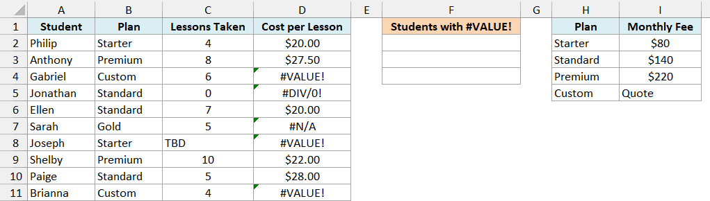
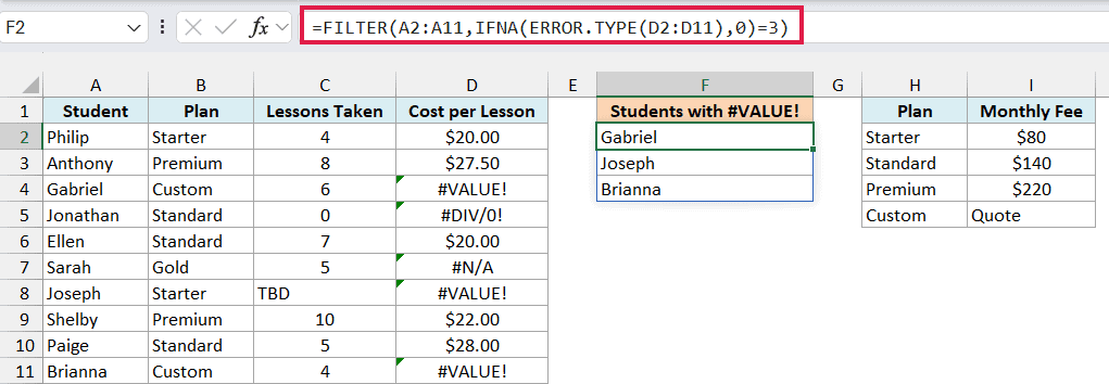
Below is a list of music students with their plan and lessons taken this month, where the cost per lesson divides the plan’s monthly fee by the lessons, and I want to list the students whose cost shows #VALUE! in column F.
Here is the formula:
=FILTER(A2:A11,IFNA(ERROR.TYPE(D2:D11),0)=3)
How this formula works:
- ERROR.TYPE(D2:D11) returns 3 for #VALUE!, 2 for #DIV/0!, 7 for #N/A, and #N/A for the rows without an error.
- IFNA(…,0) turns those “no error” #N/A values into 0, so the next check works on every row.
- =3 gives TRUE only for the #VALUE! rows, and the FILTER function returns the student names for those rows.
The result is Gabriel, Joseph, and Brianna. Gabriel and Brianna are on the Custom plan, whose fee is the text “Quote”, and Joseph’s lessons say “TBD”.
That’s the same error from two different causes, which is why it’s easier to filter by the error number than to check each cause.
Jonathan (#DIV/0!, from 0 lessons) and Sarah (#N/A, because her Gold plan isn’t in the fee list) aren’t listed, because their errors have different numbers.
Important: Keep the IFNA part. Without it, the “no error” #N/A values go straight into the FILTER function, and the formula returns #N/A instead of the list.
To list a different error, change the 3 to that error’s number. With =2, the formula returns Jonathan, the only student with a #DIV/0!.
The FILTER function only works in Excel 365 and 2021 or later.
Example 5: ERROR.TYPE With #SPILL! and #CALC! Errors
This last one covers two errors you only see in Excel 365 and 2021 or later, which most ERROR.TYPE tables leave out.
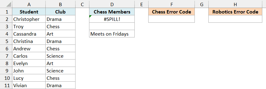
Below is a list of students and the club each one joined, with a FILTER formula in D2 that should list the Chess members, and I want the error code for D2 in cell F2.
Here is the formula:
=ERROR.TYPE(D2)
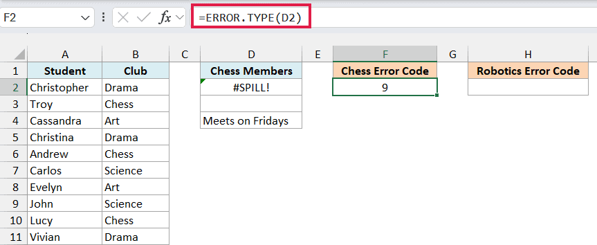
This returns 9, the number for #SPILL!. The FILTER formula in D2 needs D2:D4 for the three Chess members, but the note in D4 is in the way, so it can’t spill its results.
Now let’s check a FILTER that finds nothing at all. No student joined Robotics, and I want the error code for that FILTER in cell H2.
Here is the formula:
=ERROR.TYPE(FILTER(A2:A11,B2:B11="Robotics"))
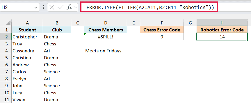
This returns 14, the number for #CALC!. The FILTER function returns #CALC! when nothing matches, and since ERROR.TYPE accepts a formula, you can check it without putting the FILTER in its own cell.
When a FILTER does sit in its own cell, such as a Robotics members list, you can give it a third argument with the value to show when nothing matches. It then never returns #CALC!, so there’s no error for ERROR.TYPE to report.
Unlike #REF! or #N/A, you can’t type #SPILL! or #CALC! straight into ERROR.TYPE, because Excel doesn’t accept them as typed values. They have to come from a cell or a formula, as they do here.
So these are some practical ways to use the ERROR.TYPE function in Excel. I covered the number for each error, hiding the #N/A for cells without errors, custom messages for each error type, filtering rows by error, and the newer #SPILL! and #CALC! errors.
I hope you found this Excel tutorial useful.
Other Excel Articles You May Also Like:
