

The PHI function in Excel returns the height of the standard normal bell curve at a given point. That height is called probability density, and you can use it to calculate the values that trace the curve.
The standard normal distribution has an average of 0 and a standard deviation of 1. PHI gives you the curve’s height at your chosen value, rather than the percentage of values below it.
Below, I’ll show you how to calculate one density, fill a list with one formula, and use PHI with values that need standardizing first.
Follow along with the example file
PHI Function Examples.xlsx
PHI Function Syntax
Here is the syntax of the PHI function:
=PHI(x)
- x (required): The number where you want the standard normal density. You can supply a number directly, reference a cell, or use a range in a version of Excel that supports spilling.
This input is often called a z-score: it tells you how many standard deviations a value sits above or below the average. Positive values are above the average, negative values are below it, and zero is at the average.
PHI is available in Excel 2013 and later. The spilling examples below use Microsoft 365, Excel 2024, or Excel 2021; single-cell alternatives are included for Excel 2013 through 2019.
When to Use the PHI Function
Use this function when you need to:
- Calculate the standard normal curve’s height at a particular z-score.
- Prepare a list of density values for a bell curve.
- Compare standardized values using the same normal curve.
Let me show you how these calculations work in Excel.
Example 1: Find Density for One Z-Score
Let’s start with one value so the result is easy to interpret.
Below is a z-score of 1.25 in cell B1, and I want its standard normal density in cell B3.
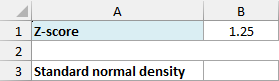
Enter this formula in cell B3:
=PHI(B1)
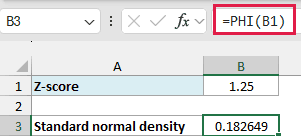
The formula returns 0.182649, displayed to six decimal places. It reads 1.25 from B1 and calculates the height of the curve at that point.
Important: A density of 0.182649 does not mean an 18.26% probability. Probabilities come from areas under the curve, so changing this result to Percentage format would give it the wrong meaning.
If the input cell contains text that Excel cannot read as a number, such as “pending”, PHI returns #VALUE!. Replace that text with the numeric z-score before calculating its density.
Example 2: Calculate a List of Densities
Now let’s calculate several points on the same curve.
Below is a list of z-scores on both sides of zero, and I want their standard normal densities in column B.
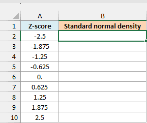
Enter this formula in cell B2:
=PHI(A2:A10)
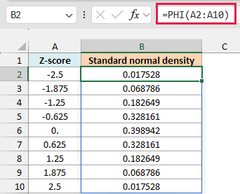
PHI calculates a density for every value in A2:A10. Press Enter once, and the nine results spill into B2:B10 without copying the formula down.
Notice that -1.25 and 1.25 both return 0.182649. The standard normal curve is symmetric, so values the same distance from zero have the same density.
Zero returns the highest density, 0.398942. As the z-scores move farther from zero in either direction, the curve gets lower and the densities get smaller.
If Excel shows #SPILL!, check that the cells below B2 are empty. Existing values in the output area stop Excel from placing all nine results there.
If you are using Excel 2013 through 2019, enter the following formula in B2 and copy it down to B10:
=PHI(A2)
Example 3: Compare Density and Probability
The difference is easier to see when both results use the same input.
Below is the z-score 1.25 again, and I want to compare PHI density, an equivalent density formula, and cumulative probability in column B.
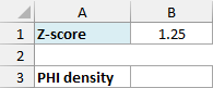
First, enter the PHI formula in B3:
=PHI(B1)
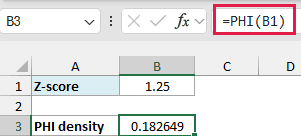
This gives the density 0.182649, as in the first example. The NORM.S.DIST function can also return density when its second argument is FALSE.
Enter this comparison formula in B4:
=NORM.S.DIST(B1,FALSE)
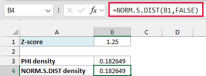
Both formulas return the same value. PHI is the shorter choice when you only need standard normal density.
To find the probability that a standard normal value is less than or equal to 1.25, enter this formula in B5:
=NORM.S.DIST(B1,TRUE)
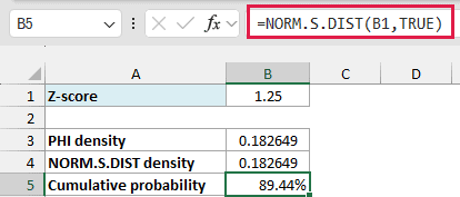
This returns about 0.894350, shown as 89.44% in the workbook. It measures the area under the curve to the left of 1.25, so Percentage format makes sense for this result.
The NORM.S.DIST function tutorial covers more probability calculations, including values above or between z-scores.
Example 4: Standardize Delivery Times First
Your starting numbers won’t always be z-scores.
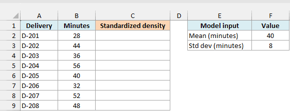
Suppose delivery times follow a normal model with a mean of 40 minutes and a standard deviation of 8 minutes. These are supplied model parameters, not statistics calculated from the eight deliveries below.
Below are eight delivery durations, and I want the standard normal density of each delivery’s z-score in column C.
Enter this formula in cell C2:
=PHI((B2:B9-$F$2)/$F$3)
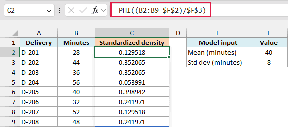
The formula subtracts the mean in F2 from every delivery time, then divides each difference by the standard deviation in F3. That converts the durations to z-scores before PHI calculates their densities.
For the 28-minute delivery, the calculation is (28 – 40) / 8, which gives a z-score of -1.5. PHI returns 0.129518, and the result spills into the first output cell.
The 52-minute delivery is equally far above the mean, so it returns the same density. The 40-minute delivery is exactly at the mean and returns the highest density, 0.398942.
Make sure F3 contains a positive standard deviation. Zero causes a division error, while a negative value is not a valid standard deviation even if this arithmetic formula returns a number.
Important: These results are densities on the standardized z-score scale, not densities per minute. If you need density on the original time scale, use the NORM.DIST function with your mean, standard deviation, and FALSE.
If you are using Excel 2013 through 2019, enter this formula in C2 and copy it down to C9:
=PHI((B2-$F$2)/$F$3)
The dollar signs keep the model inputs fixed while the delivery-time reference changes as you copy the formula.
You can now use PHI with a single z-score or a whole list, including values you standardize first. Keep density separate from probability when interpreting the results.
Other Excel Articles You May Also Like:
