

The RSQ function in Excel returns the R-squared value (also called the coefficient of determination) for two sets of numbers. It’s a number between 0 and 1 that tells you how well a straight line fits your data.
You can read it as the share of the change in one value that’s explained by the other. So an R-squared of 0.80 means 80% of the ups and downs in one column line up with the other column.
In this article, I’ll show you how to use RSQ to find R-squared, how to read the result, and how to use it to compare factors, groups, and even a curved trend.
Follow along with the example file
RSQ Function Examples.xlsx
RSQ Function Syntax
Here is the syntax of the RSQ function:
=RSQ(known_y's, known_x's)
- known_y’s – The values you want to explain, such as rent or sales.
- known_x’s – The values you think explain them, such as size or ad spend. It needs the same number of cells as known_y’s.
RSQ pairs the two ranges by position, so the first value in known_y’s goes with the first value in known_x’s, the second with the second, and so on.
Swapping the two ranges gives the same result. It’s still a good habit to put the values you want to explain first, because that’s how the argument names read.
If either value in a pair is a blank cell, text, or TRUE/FALSE, RSQ skips that whole pair. A zero is a real number, though, so a pair with a 0 stays in the calculation.
The RSQ function works in all Excel versions, including Microsoft 365, Excel 2024, 2021, 2019, 2016, and Excel for Mac.
When to Use the RSQ Function
Use this function when you need to:
- Find the R-squared value between two columns of numbers
- Check how well a straight trend line fits your data
- Compare which of two factors explains a result better
- Get the R-squared for each group in a dataset
- Check whether a growth curve fits your data better than a straight line
Let me show you five practical examples of how to use the RSQ function.
Example 1: Find R-Squared in Excel Using RSQ
Let’s start with a simple example.
Below is a list of apartments with their size in square feet and monthly rent, and I want to find how well the size explains the rent in cell F1.
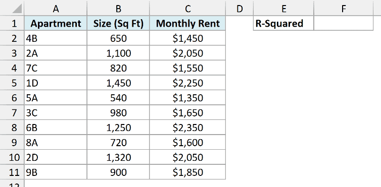
Here is the formula:
=RSQ(C2:C11,B2:B11)
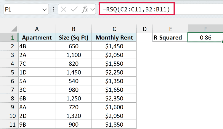
This gives 0.86. The rent in C2:C11 is the value I want to explain, so it goes first, and the size in B2:B11 goes second.
An R-squared of 0.86 means about 86% of the differences in rent between these apartments line up with their size. The other 14% comes from things the size doesn’t capture, like the floor or the view.
The closer the result is to 1, the more tightly the points sit around a straight line. A result close to 0 means a straight line doesn’t explain much at all.
If you plot these two columns in a scatter plot and add a linear trendline with its R-squared value shown, the chart shows 0.8637, the same number RSQ gives you.
Important: If the two ranges don’t have the same number of cells, RSQ returns the #N/A error. A common cause is selecting the header in one range but not the other, as in =RSQ(C2:C11,B1:B11).
You’ll get the #DIV/0! error if a range has only one number in it, or if one of the columns has the same value in every row. In both cases, there’s no variation for RSQ to compare.
Example 2: Compare Which Factor Explains a Result Better
Now let’s use RSQ to compare two factors.
Below is a list of restaurant bills with the bill amount, the party size, and the tip for each table, and I want to see which of the two explains the tip better in cells G1 and G2.
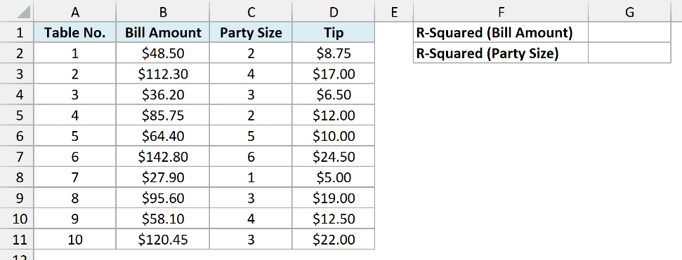
Here is the formula for the bill amount in cell G1:
=RSQ(D2:D11,B2:B11)
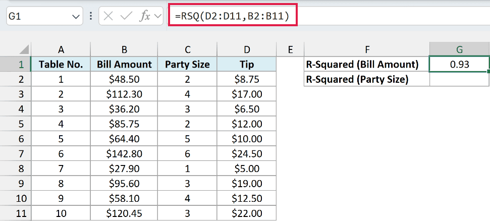
This gives 0.93, so about 93% of the differences in tips line up with the size of the bill.
And here is the formula for the party size in cell G2:
=RSQ(D2:D11,C2:C11)
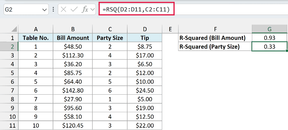
This gives 0.33, so the party size explains only about a third of the differences in tips.
Both formulas use the tips in D2:D11 as the first range, because that’s the value we’re trying to explain. Only the second range changes.
So the bill amount is a much better guide to the tip than the party size. That makes sense, since most people work out a tip as a share of the bill.
Keep in mind that a high R-squared shows two things move together. It doesn’t prove that one causes the other.
Example 3: RSQ vs CORREL (R-Squared Doesn’t Show Direction)
Here’s something about RSQ that can catch you out.
Below is a list of laptops with each laptop’s age in years and how long its battery lasts on a full charge, and I want the R-squared in cell F1 and the correlation in cell F2.
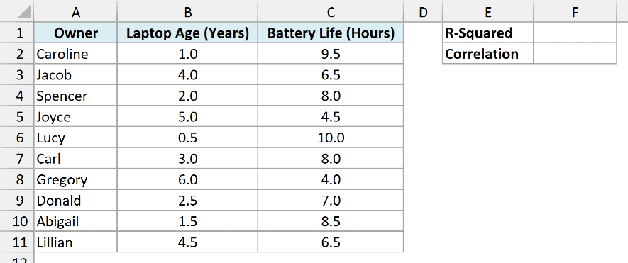
Here is the formula for R-squared:
=RSQ(C2:C11,B2:B11)
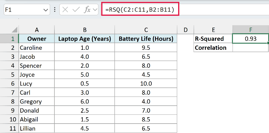
This gives 0.93, so laptop age explains about 93% of the differences in battery life.
But the number doesn’t tell you whether battery life goes up or down as laptops get older. R-squared is always between 0 and 1, so it never has a minus sign.
To see the direction, here is the formula with the CORREL function in cell F2:
=CORREL(C2:C11,B2:B11)
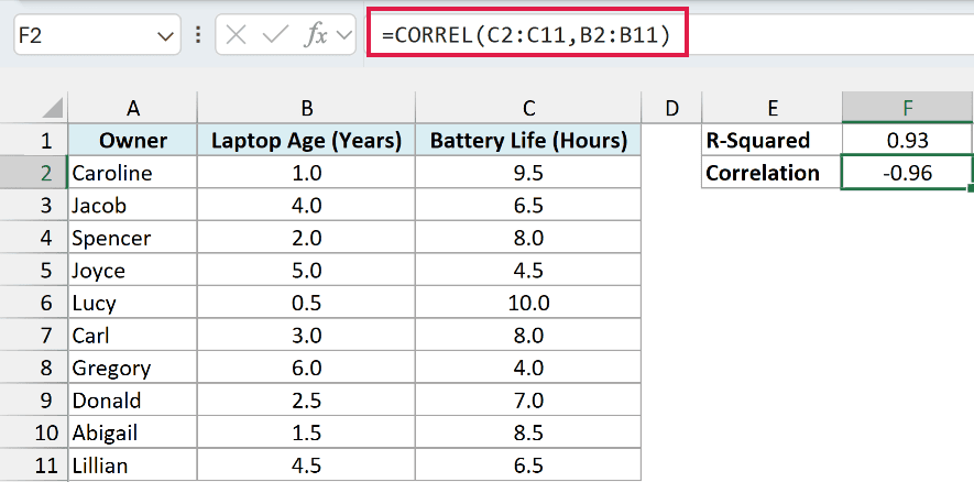
This gives -0.96. The minus sign means the two move in opposite directions, so older laptops have shorter battery life.
RSQ is the square of this correlation. If you square -0.96 (more precisely -0.9618), you get 0.93, which is why the sign disappears.
So use the CORREL function (or the PEARSON function, which gives the same result) when you need to know the direction. Use RSQ when you want to know how much of the change one value explains.
Example 4: Get R-Squared for Each Group With One Formula
Let’s step it up with one formula that gives a separate R-squared for each group.
Below is a list of ride-share trips with the city, the miles traveled, and the fare, and I want the R-squared between miles and fare for each city in column F.
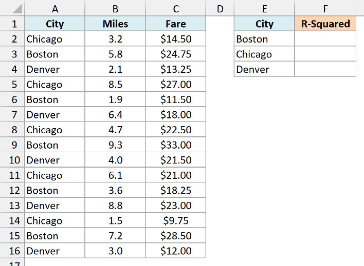
Here is the formula in cell F2:
=MAP(E2:E4,LAMBDA(city,RSQ(FILTER(C2:C16,A2:A16=city),FILTER(B2:B16,A2:A16=city))))
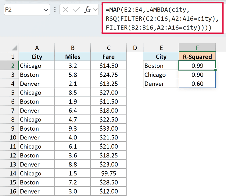
This spills three results into F2:F4. It gives 0.99 for Boston, 0.90 for Chicago, and 0.60 for Denver.
How this formula works:
- MAP(E2:E4,…) goes through the city names in E2:E4 one at a time.
- LAMBDA(city,…) gives the current city name the name city.
- FILTER(C2:C16,A2:A16=city) keeps only the fares for that city, and FILTER(B2:B16,A2:A16=city) keeps only its miles.
- RSQ then finds the R-squared for just those trips, and each result lands next to its city.
So in Boston and Chicago, the distance explains most of the fare. In Denver, it explains only about 60%, which tells you something other than the miles is also moving the fare there.
If you used RSQ on all 15 trips together, you’d get 0.79, which hides how different Denver is from the other two cities.
The MAP function and the LAMBDA function are available in Excel 365 and Excel 2024. The FILTER function is available in Excel 365, 2024, and 2021.
If you are using Excel 2021 or earlier, enter the below formula in cell F2 and then copy it down to F4:
=RSQ(IF($A$2:$A$16=E2,$C$2:$C$16,""),IF($A$2:$A$16=E2,$B$2:$B$16,""))
The IF function turns the trips from other cities into empty text, and RSQ skips text, so only the matching city’s trips are used. In Excel 2019 or earlier, enter it with Control + Shift + Enter instead of just Enter.
Example 5: Check If a Growth Curve Fits Better Than a Straight Line
Finally, let’s use RSQ to check the shape of a trend.
Below is the number of newsletter subscribers at the end of each month in 2025, and I want the R-squared for a straight-line trend in cell F1 and for an exponential (growth) trend in cell F2.
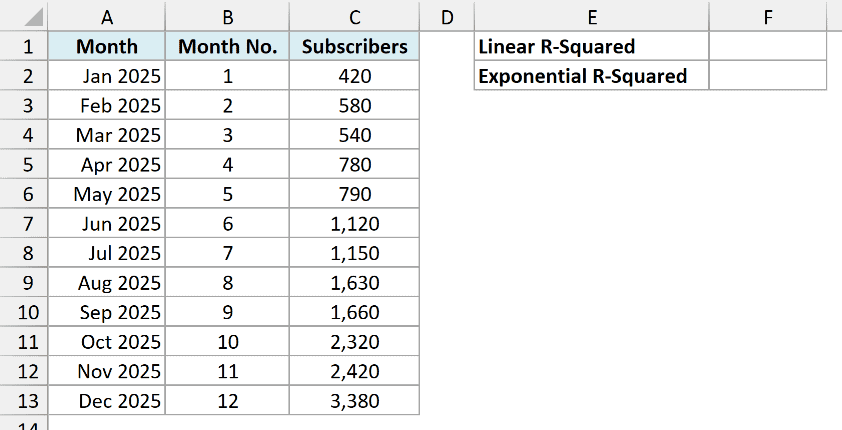
Here is the formula for the straight-line trend:
=RSQ(C2:C13,B2:B13)
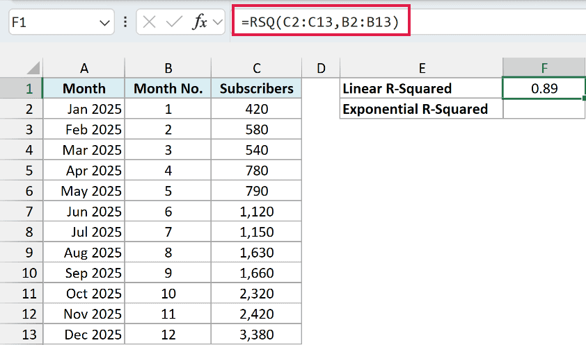
This gives 0.89.
The Month No. column in B2:B13 is the x value here. I’m using 1 to 12 instead of the dates because months have different numbers of days, which would space the points slightly unevenly.
RSQ against the month numbers gives the same result as comparing the actual subscribers with the values a straight line predicts for each month. That’s also the 0.89 Excel shows when you add a linear trendline to a chart of this data.
That looks like a pretty good fit, but the subscribers grow faster as the year goes on, so the numbers actually curve upward.
To check a growth curve instead, you can give RSQ the values the curve predicts. Here is the formula in cell F2:
=RSQ(C2:C13,GROWTH(C2:C13,B2:B13))
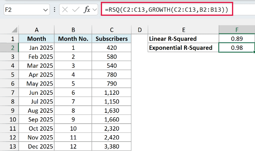
This gives 0.98, so the growth curve fits the data much better than a straight line.
How this formula works:
- GROWTH(C2:C13,B2:B13) fits an exponential curve to the data and returns the predicted subscribers for each of the 12 months.
- RSQ uses those 12 predicted values as its known_x’s and checks how closely they line up with the actual subscribers in C2:C13. The better they line up, the closer the result is to 1.
The 0.98 matches the R-squared Excel shows when you add an exponential trendline to the chart (0.9799).
Since both formulas compare the actual subscribers with predicted values, you can compare the 0.89 and the 0.98 directly.
If you get the R-squared for an exponential fit from the LOGEST function instead, you’ll see a slightly different value (0.9815 here). That’s because the LOGEST function measures the fit on the logarithm of the subscriber numbers.
So a decent R-squared for a straight line doesn’t mean a straight line is the right shape. When your data grows by a percentage each period, check a curve too.
The GROWTH function is the one that fits that kind of curve.
So these are five ways to use the RSQ function in Excel. RSQ works with one set of x values, so if you need R-squared for a model with several factors, the LINEST function can give you that.
I hope you found this article helpful.
Other Excel Articles You May Also Like:
