

The BESSELY function returns the Bessel function of the second kind, Yn(x), also known as the Weber or Neumann function. It’s one of four Bessel functions in the engineering category of Excel functions.
Bessel functions show up in physics and engineering problems built around circles and cylinders, like a vibrating drumhead or waves in a pipe.
You don’t need the math to use it. You give BESSELY a number x and a whole-number setting called the order n, and it returns one point on a wavy curve.
The catch is that x has to be greater than 0, a decimal order gets cut down to a whole number, and BESSELY won’t take a range of cells directly. The examples below show all three.
Follow along with the example file
BESSELY Function Examples.xlsx
BESSELY Function Syntax
Here is the syntax of the BESSELY function:
=BESSELY(x, n)
- x – The point on the curve that you want the value for. It has to be greater than 0, or BESSELY returns the #NUM! error.
- n – The order, a whole number like 0, 1, or 2 that picks which curve you get. Y0 and Y1 give different results for the same x, and n can’t be negative.
Both arguments have to be numbers. If either one is text, BESSELY returns the #VALUE! error, and a negative n returns the #NUM! error.
The BESSELY function works in Excel 2016 and later, including Excel 2019, 2021, 2024, and Microsoft 365, on Windows and Mac.
When to Use the BESSELY Function
Use the BESSELY function when you need to:
- Get the value of Yn(x) for a physics or engineering formula that involves a circle or a cylinder.
- Build a table of Yn(x) values for different x values or orders.
- Find roughly where Yn(x) crosses zero.
- Check a hand calculation or a printed Bessel table against Excel.
Let me show you a few examples of how it works.
Example 1: Get a Single BESSELY Value
Let’s start with the simplest case, one x and one order.
Below I have a small card with the value of x and the order n, and I want to get the BESSELY value in cell B4.
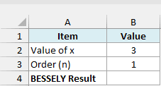
Here is the formula:
=BESSELY(B2,B3)
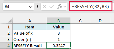
Here x is 3 and n is 1, so the formula returns Y1(3), which is about 0.3247. Change the number in B2 or B3 and the result updates.
A single BESSELY value is just one point on a wavy curve that swings above and below zero as x grows. The next examples show more of that curve.
Example 2: Get BESSELY Values for a List of x Values
Now let’s calculate a whole column of values with one formula.
Below I have a list of x values in column A, and I want to get the order 0 BESSELY value for each one in column B.
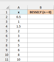
Here is the formula:
=BESSELY(A2:A11+0,0)
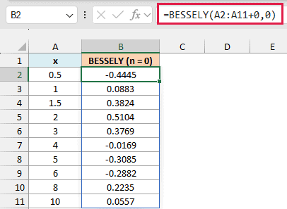
The formula spills down column B, so you enter it once in B2 and Excel fills the rest. The 0 at the end is the order, so every x gets its Y0 value.
The +0 after the range doesn’t change any value, but it makes Excel pass the numbers as a list that BESSELY can work through.
Important: If you pass a range like A2:A11 straight to BESSELY, you get one #VALUE! error and nothing spills, even in Excel 365. Keep the +0 after every range you give it.
A few other functions, like EOMONTH and WORKDAY, refuse a range in the same way. I explain why in my guide on Excel functions that won’t spill.
Look at how the results behave. They start negative at x = 0.5, turn positive, dip negative again between 4 and 6, and then swing back up, with the swings getting smaller as x grows.
If you are using Excel 2019 or earlier, enter the below formula in cell B2 and then copy it down the range:
=BESSELY(A2,0)
Example 3: Compare Several Orders in One Grid
Next, let’s put different orders side by side.
Below I have x values down column A and the orders 0 to 3 across row 1, and I want to get the BESSELY value for every x and order pair in columns B to E.
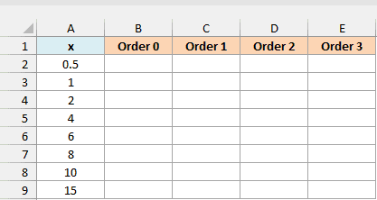
Here is the formula:
=BESSELY(A2:A9+0,B1:E1+0)
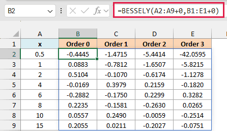
One formula fills the whole grid. Excel pairs each x in column A with each order in row 1, so you get 32 results from a single formula in B2.
Read across the first row, where x is 0.5. The values go from about -0.44 for order 0 to about -42.06 for order 3, so higher orders start much further below zero.
Pro Tip: The headers in B1:E1 are plain numbers (0, 1, 2, 3) with the custom number format “Order “0, which is why the formula can use them as the order.
If you are using Excel 2019 or earlier, enter the below formula in cell B2 and then copy it across to column E and down to row 9:
=BESSELY($A2,B$1)
Example 4: Decimal Orders Are Cut Down to Whole Numbers
Let’s see what happens when the order isn’t a whole number.
Below I have a list of orders in column A and the value of x in cell E1, and I want to get the BESSELY value for each order in column B.
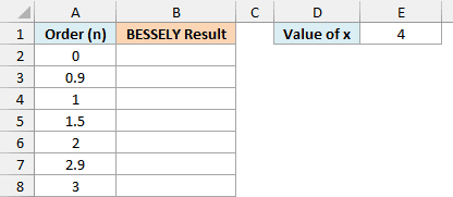
Here is the formula:
=BESSELY(E1,A2:A8+0)
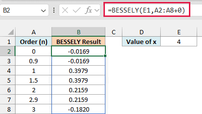
Excel drops the decimal part of the order instead of rounding it. So an order of 0.9 gives the same result as 0, 1.5 gives the same result as 1, and 2.9 gives the same result as 2.
That means 2.9 doesn’t round up to 3. If you want order 3, you have to type 3.
Example 5: BESSELY Near Zero and the #NUM! Error
Now let’s see what happens as x gets close to zero.
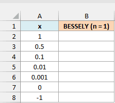
Below I have a list of x values that get smaller and smaller, ending with 0 and a negative number, and I want to get the order 1 BESSELY value for each one in column B.
Here is the formula:
=BESSELY(A2:A8+0,1)
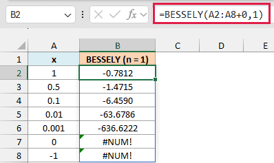
Each time x gets 10 times smaller, the result gets about 10 times further below zero. It goes from about -6.46 at 0.1 to -63.68 at 0.01 and -636.62 at 0.001.
Yn(x) keeps dropping toward negative infinity as x approaches 0, so Excel can’t give you a number at x = 0. That’s why BESSELY returns the #NUM! error for the 0 in A7.
The -1 in A8 returns the same error, because BESSELY only accepts an x that is greater than 0.
Example 6: Find Where BESSELY Crosses Zero
Let’s finish with something practical, finding where the curve crosses zero.
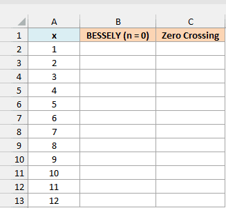
Below I have a list of x values from 1 to 12, and I want to get the order 0 BESSELY value for each one in column B.
Here is the formula:
=BESSELY(A2:A13+0,0)
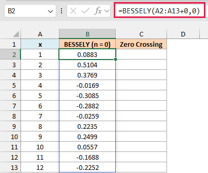
Now I want to flag every pair of neighboring x values where the result changes sign, because the curve must cross zero somewhere between them.
Enter this formula in cell C2 and it spills down the column:
=IF(B2:B12*B3:B13<0,"Between "&A2:A12&" and "&A3:A13,"")
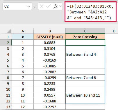
The formula multiplies each result in B2:B12 by the one below it in B3:B13. A negative product means one is positive and the other is negative, so the formula returns text like Between 3 and 4.
The curve crosses zero between 3 and 4, between 7 and 8, and between 10 and 11. Use a smaller step between x values, like 0.1, to narrow each crossing down further.
So that’s how you can use the BESSELY function in Excel. Just keep x above 0, stick to whole-number orders, and add +0 after any range you give it.
I hope you found this Excel tutorial useful.
Other Excel Articles You May Also Like:
