
To use XLOOKUP with multiple criteria, you combine your conditions into something one lookup value can find. XLOOKUP only takes a single lookup value, so this small workaround is what lets it match on two, three, or more columns.
In this article, I’ll show you three ways to do it, starting with the one I recommend. I’ll also cover greater-than conditions, either-or conditions, finding the latest match, and what to do when nothing matches.
Follow along with the example file
XLOOKUP Multiple Criteria Examples.xlsx
XLOOKUP with Multiple Criteria Using Boolean Logic (Recommended)
This method needs no extra columns, and it works with as many conditions as you want.
You check each condition against its own column, which gives you a list of TRUE and FALSE values (that’s the boolean part). Then you multiply those lists and look for the row that comes out as 1.
Let me show you how it works.
Below is a sales summary with the total sales for each region and product, and I want to get the sales in F3 for the region in F1 and the product in F2.
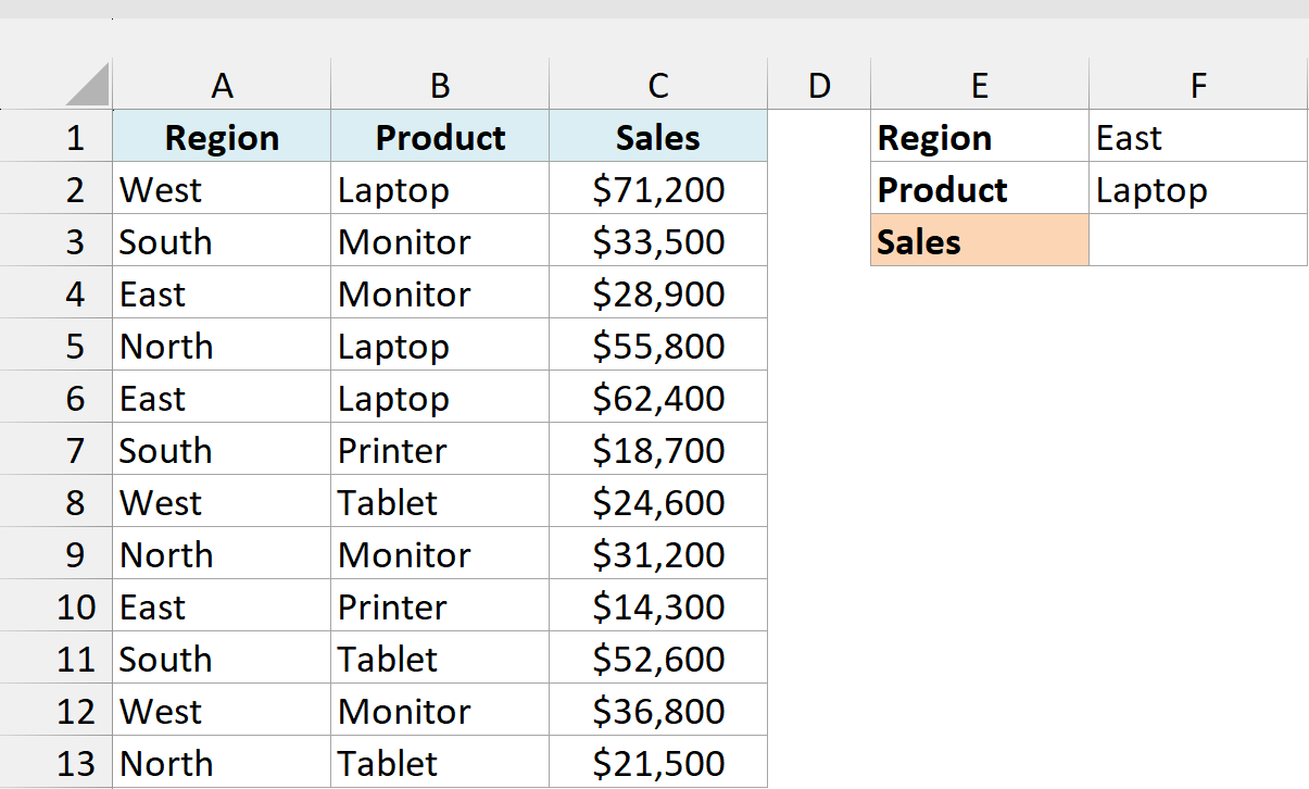
Here is the formula that will give us the result:
=XLOOKUP(1,(A2:A13=F1)*(B2:B13=F2),C2:C13)
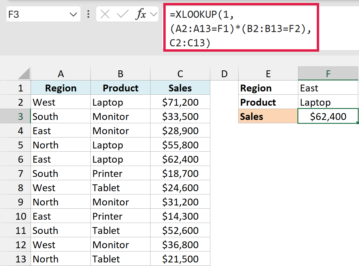
How does this formula work?
(A2:A13=F1) checks every region against East and gives back a list of TRUE and FALSE values. (B2:B13=F2) does the same thing for the product, using Laptop.
When you multiply the two lists, Excel treats TRUE as 1 and FALSE as 0. So a row only ends up as 1 when both conditions are true, and every other row becomes 0.
The formula then looks for that 1. It’s in row 6 (East, Laptop), so XLOOKUP returns the sales from that row, which is $62,400.
A regular XLOOKUP on the region alone would stop at the first East row. That’s row 4, Monitor sales of $28,900, which is why you need both conditions here.
You only need to press Enter after typing this formula. There’s no need for Control + Shift + Enter, even though the formula is working through whole lists of values.
The XLOOKUP function works in Excel 365, 2024, and 2021. It’s not available in Excel 2019 or earlier.
If you’re on an older version of Excel, you can do the same lookup with INDEX MATCH with multiple criteria instead.
XLOOKUP with Three or More Criteria
To add another condition, you multiply one more check into the same formula. The structure stays the same, because each new condition is just one more set of brackets.
Below is a sales summary that’s split by quarter, and I want to get the sales in G4 for the region in G1, the product in G2, and the quarter in G3.
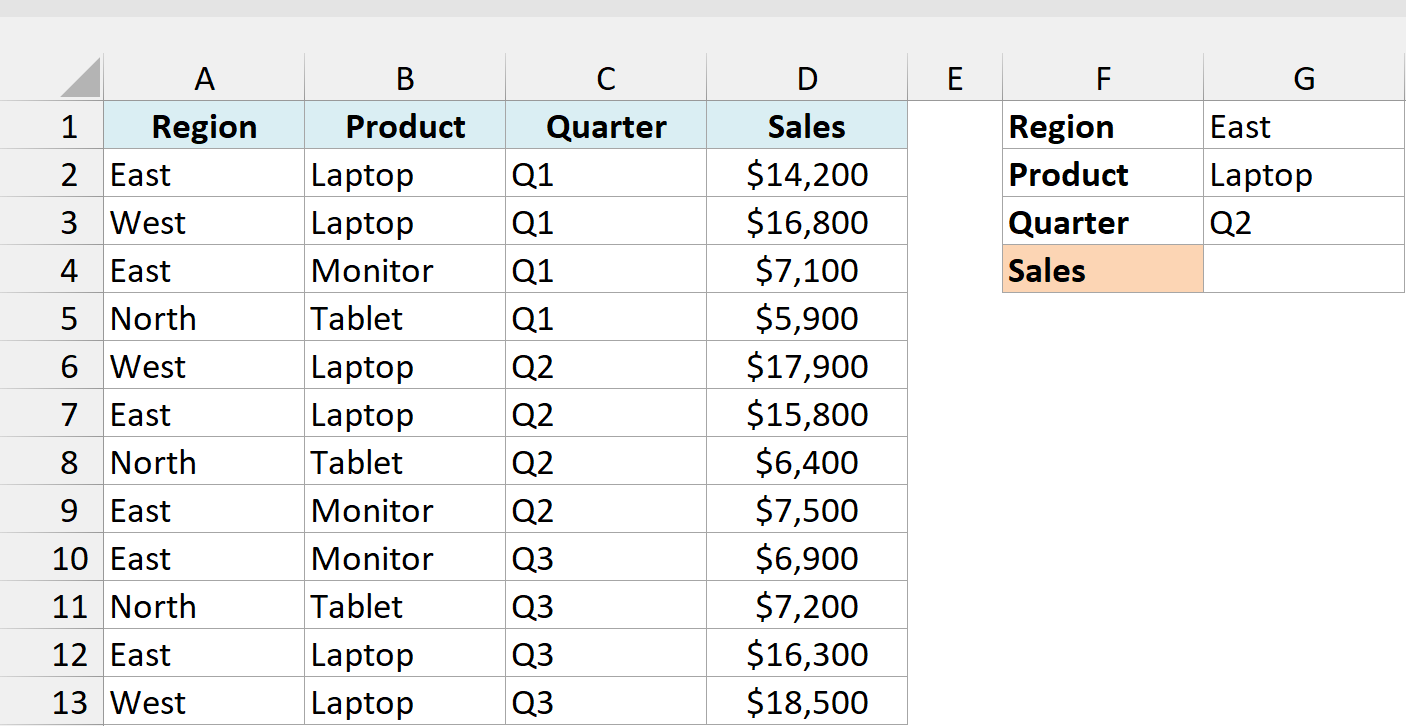
Here is the formula that will give us the result:
=XLOOKUP(1,(A2:A13=G1)*(B2:B13=G2)*(C2:C13=G3),D2:D13)
Row 7 (highlighted below) is the only East Laptop row for Q2.
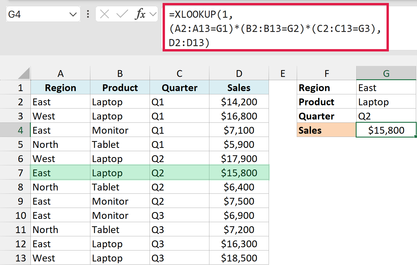
How does this formula work?
Now three lists get multiplied together, so a row only ends up as 1 when the region, the product, and the quarter all match.
That’s row 7 (East, Laptop, Q2), so the formula returns $15,800. Notice that rows 2 and 12 are also East Laptop sales, but they’re for Q1 and Q3, so they get a 0 and are skipped.
Compared with the first formula, the input cells moved from column F to G and the sales range moved from C to D. That’s only because this data has the extra Quarter column.
Use Greater Than or Less Than Conditions in XLOOKUP
A condition doesn’t have to be an exact match. You can use >, <, >=, <=, or <> inside the brackets, and the structure of the formula stays the same.
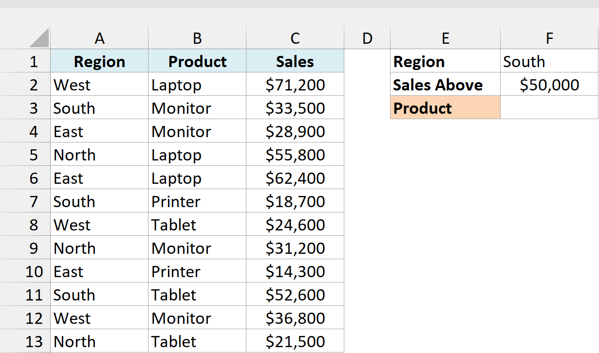
Below is the sales summary again, and I want to find which product sold more than the amount in F2 in the region in F1, with the answer in F3.
Here is the formula that will give us the result:
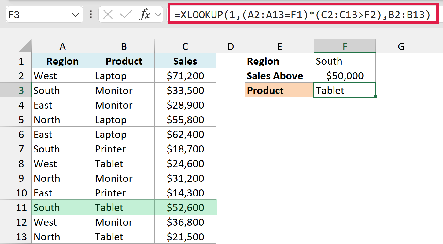
=XLOOKUP(1,(A2:A13=F1)*(C2:C13>F2),B2:B13)
Row 11 (highlighted below) is the only South row with sales above $50,000.
How does this formula work?
(C2:C13>F2) gives TRUE for every row with sales above $50,000, and (A2:A13=F1) gives TRUE for every South row. Multiplying them leaves a 1 only on the rows where both are true.
Only row 11 qualifies here (South, Tablet, $52,600), so the formula returns Tablet. The other South rows, Monitor and Printer, sold less than $50,000.
XLOOKUP picks by position only, not by which product sold the most. If more than one row passes the test, it returns the one nearest the top and doesn’t tell you about the rest.
If you want every matching row rather than just one of them, have a look at how to look up and return multiple values in one cell.
XLOOKUP with OR Logic (Either Criterion Can Match)
So far, every condition had to be true. If a row only needs to meet one of your conditions, you add the checks instead of multiplying them.
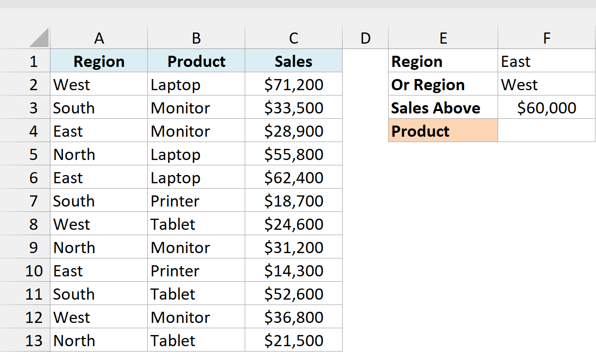
Below is the sales summary, and I want to find a product that sold more than the amount in F3 in either the region in F1 or the region in F2, with the answer in F4.
Here is the formula that will give us the result:
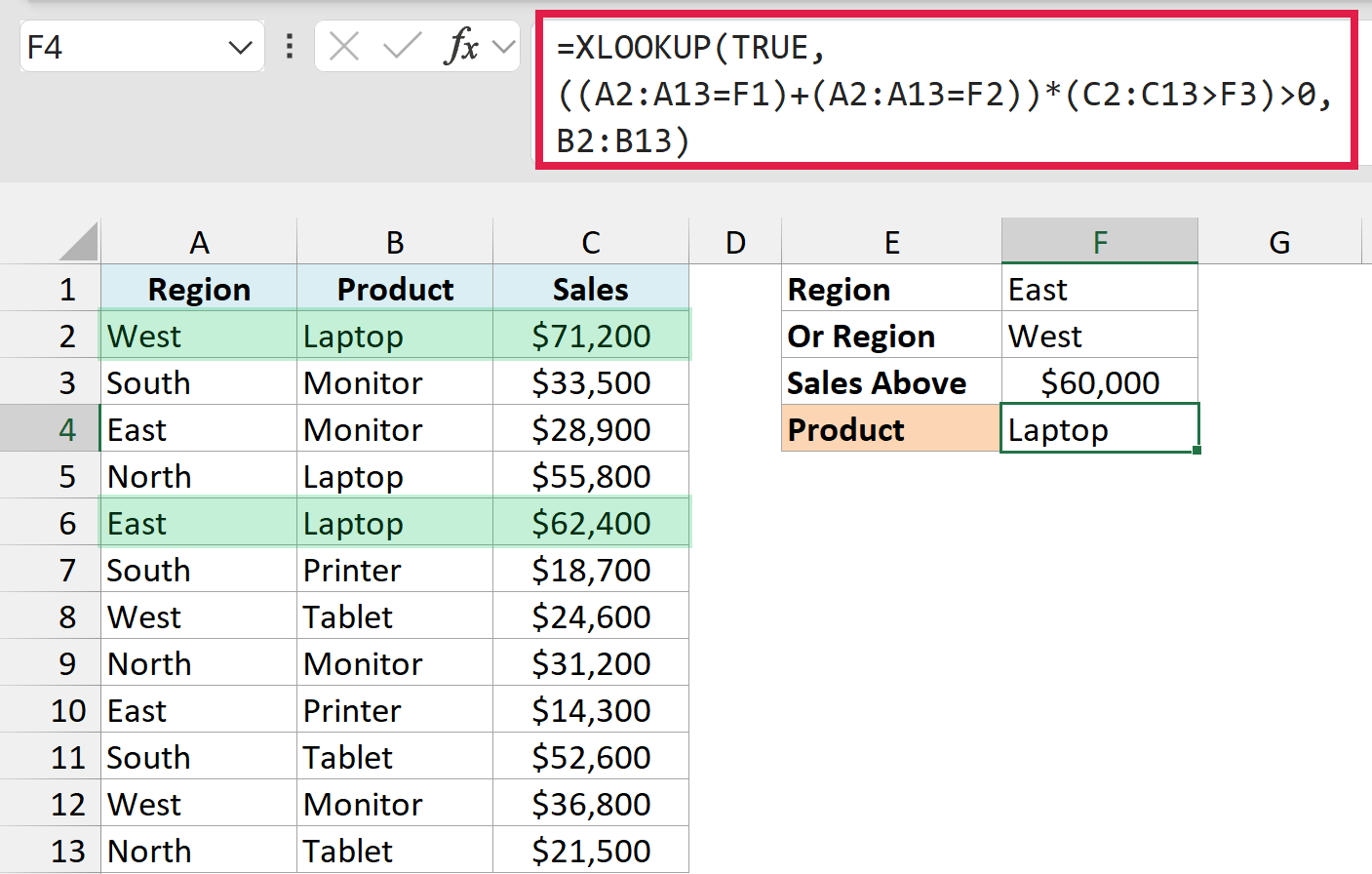
=XLOOKUP(TRUE,((A2:A13=F1)+(A2:A13=F2))*(C2:C13>F3)>0,B2:B13)
Rows 2 and 6 (highlighted below) are the East or West rows with sales above $60,000.
How does this formula work?
Adding the two region checks gives each row a score: 1 if it’s in East or West, and 0 if it’s in neither. That score is then multiplied by the sales check, so only East or West rows with sales above $60,000 stay above zero.
The >0 part turns any score above zero into TRUE, and XLOOKUP looks for the first TRUE. Two rows qualify, West Laptop in row 2 and East Laptop in row 6, and both are Laptop, so the formula returns Laptop.
The checks you add don’t have to be on the same column. With an OR across two columns, such as region West or product Laptop, a row can match both checks and score 2.
Important: Don’t look up 1 when you add checks. A row that scores 2 gets skipped, so the formula can return a later row’s value, or #N/A, without any warning.
For example, <code>=XLOOKUP(1,(A2:A13=”West”)+(B2:B13=”Laptop”),C2:C13)</code> skips row 2 (West, Laptop), which scores 2. It returns $55,800 from row 5 (North, Laptop) instead of $71,200.
Find the Latest Match with Multiple Criteria
By default, XLOOKUP searches from the top and returns the first match. When your data is a log that keeps growing, the newest entry sits at the bottom, and that’s usually the one you want.
Below is a price-change log for products from two suppliers, sorted by date, and I want to get the original price in G3 and the current price in G4 for the product in G1 and the supplier in G2.
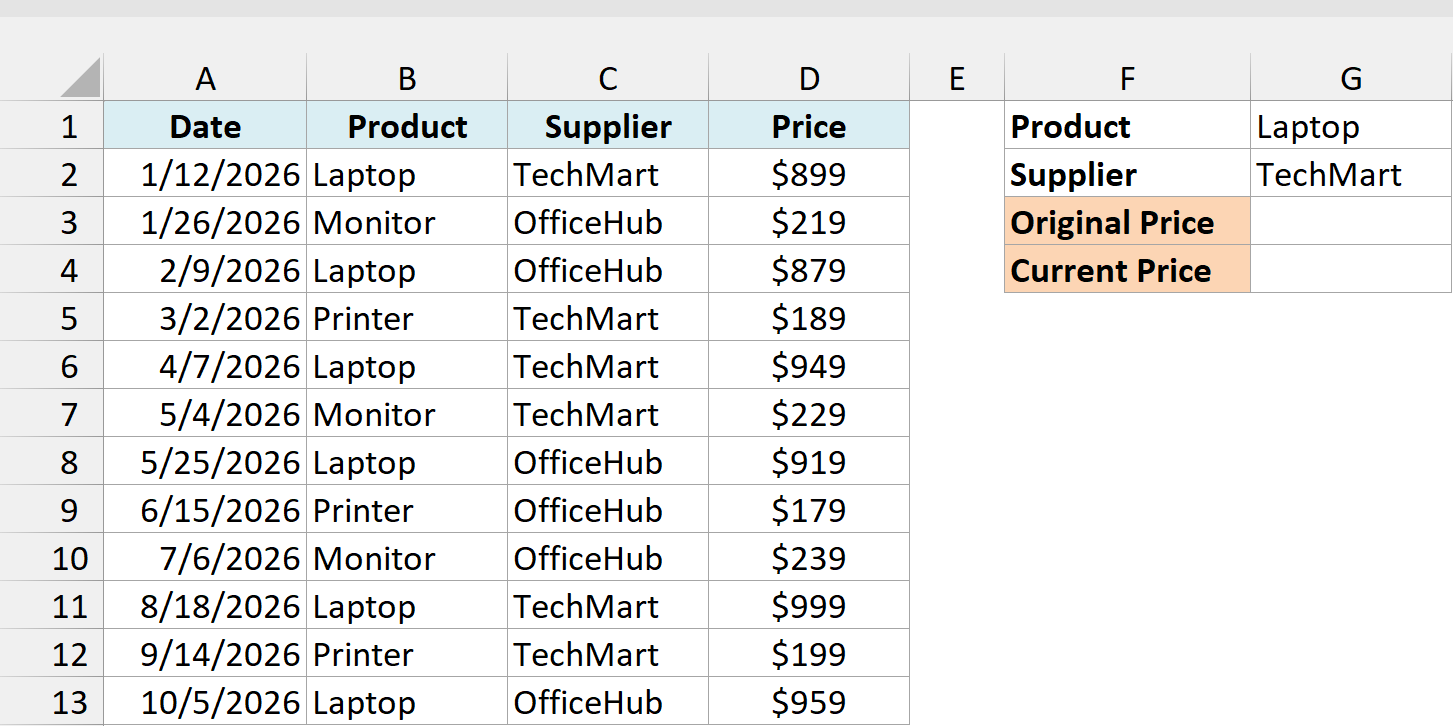
Here is the formula that gives the original price:
=XLOOKUP(1,(B2:B13=G1)*(C2:C13=G2),D2:D13)
The three TechMart Laptop entries, in rows 2, 6, and 11, are highlighted below.
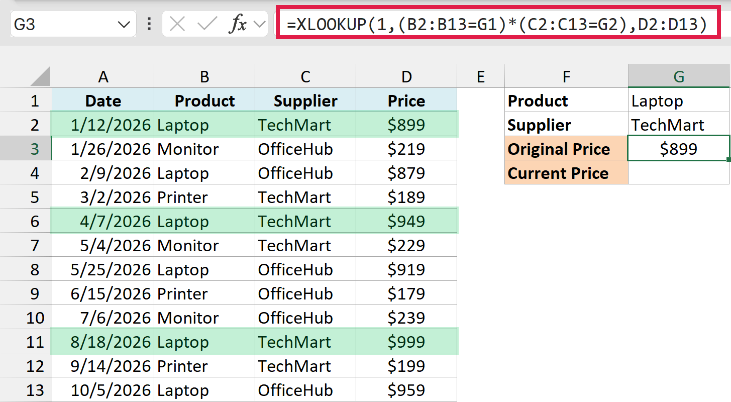
XLOOKUP searches from the top, so it stops at row 2 and returns $899, the price from January.
To get the current price, set the search mode argument to -1 so XLOOKUP searches from the bottom up. Search mode is the sixth argument, so the two empty slots before it skip if_not_found (what to show when nothing matches) and match mode:
=XLOOKUP(1,(B2:B13=G1)*(C2:C13=G2),D2:D13,,,-1)
The same three rows are highlighted below, and this time the formula picks the bottom one.
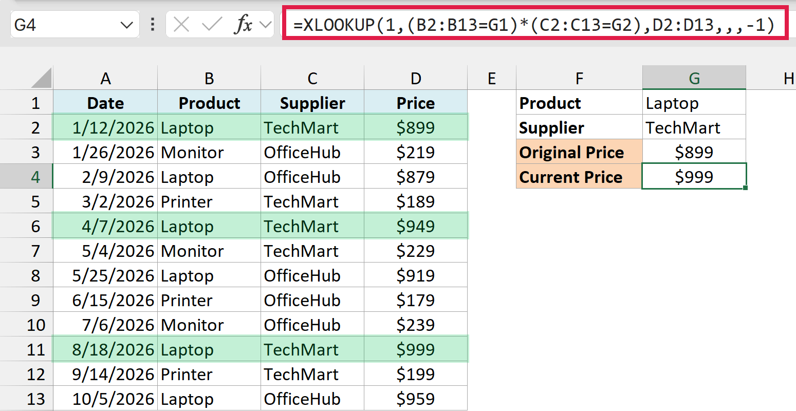
This one starts at row 13, which is a Laptop from OfficeHub, so it’s skipped. The first match from the bottom is row 11, so the formula returns $999, the price from August.
Without the supplier condition, the formula would return $959 from that OfficeHub row instead, which is why you need both conditions here.
Important: Search mode -1 means the last row, not the latest date. If your log is sorted with the newest entries at the top, the two formulas swap their results.
If your log isn’t kept in date order, use the below formula in G4 instead of the search mode one. It isn’t in the example file, so type it in if you want to try it:
=XLOOKUP(1,(B2:B13=G1)*(C2:C13=G2)*(A2:A13=MAXIFS(A2:A13,B2:B13,G1,C2:C13,G2)),D2:D13)
The MAXIFS function finds the latest date for Laptop from TechMart, which is 8/18/2026. The third check keeps only the row with that date, so the formula returns $999 no matter how the log is sorted.
Show a Message When There’s No Match
When no row meets all your conditions, the formula returns a #N/A error. You can show your own message instead by using the if_not_found argument, which is the fourth argument in XLOOKUP.
Below is the sales summary, and I want to get the sales in F3 for the region in F1 and the product in F2, but there’s no Printer sale in the North region.
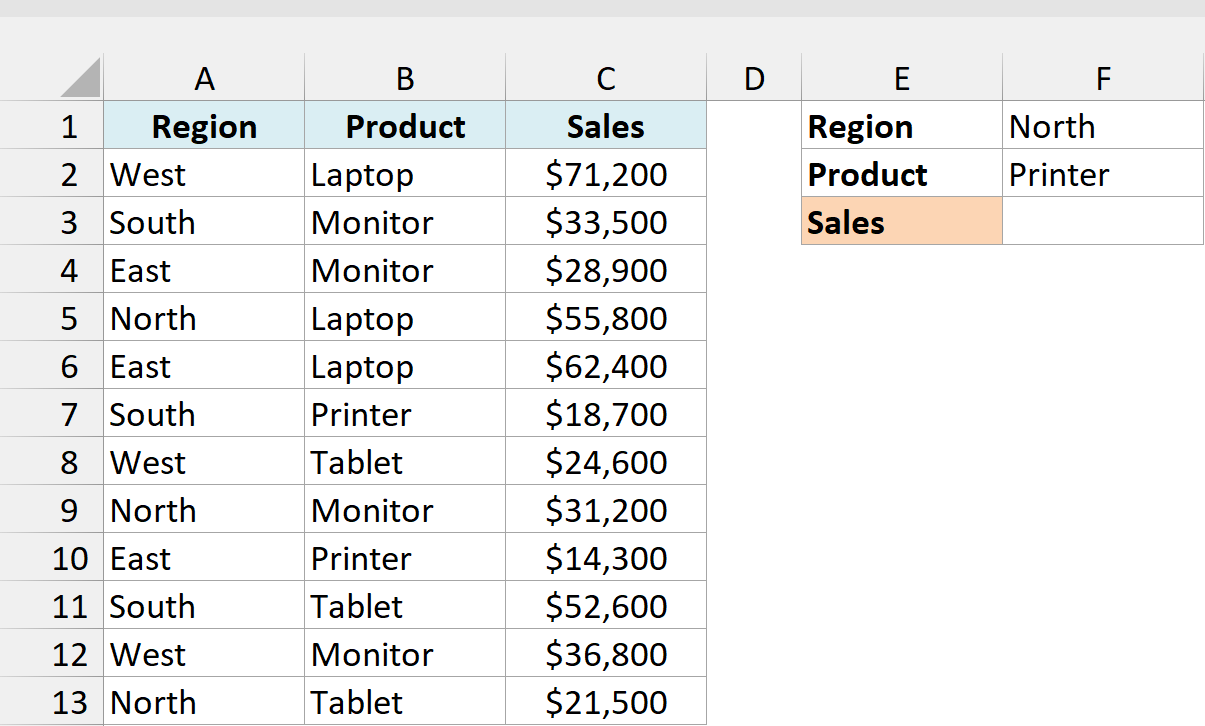
Here is the formula that will give us the result:
=XLOOKUP(1,(A2:A13=F1)*(B2:B13=F2),C2:C13,"Not found")
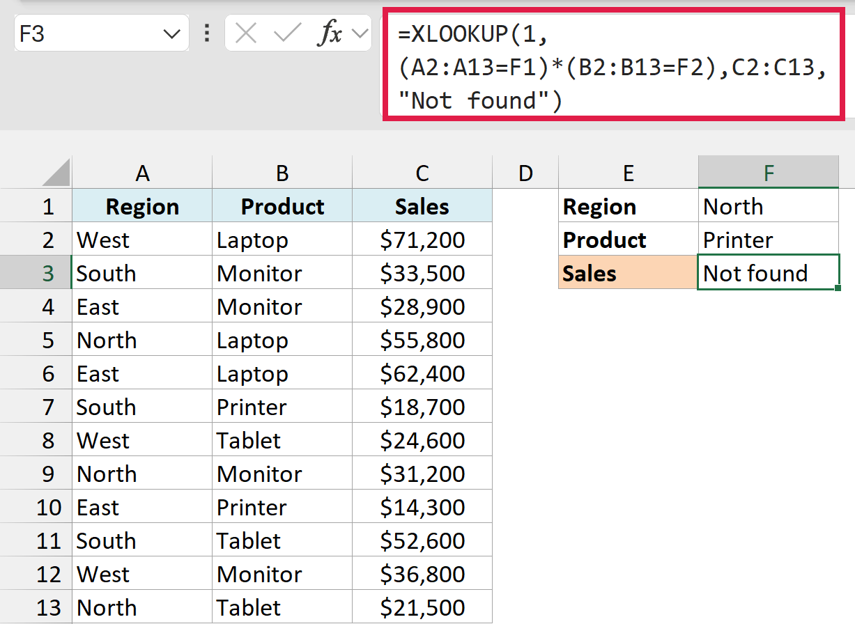
No row ends up as 1 here, so the formula returns the text Not found instead of the error.
If you get this result for a row you can clearly see in your data, check for extra spaces. These comparisons ignore upper and lower case, so east matches East, but “East ” with a trailing space doesn’t.
XLOOKUP with Multiple Criteria Using Concatenation
Here’s a second way to match on multiple criteria, if you’d rather not multiply lists of TRUE and FALSE. You join your criteria into one text value (that’s the concatenation part), join the columns the same way, and then run a normal lookup on the joined text.
Below is the sales summary with the total sales for each region and product, and I want to get the sales in F3 for the region in F1 and the product in F2.
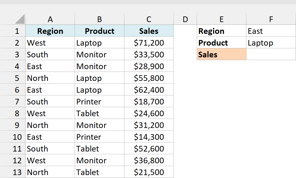
Here is the formula that will give us the result:
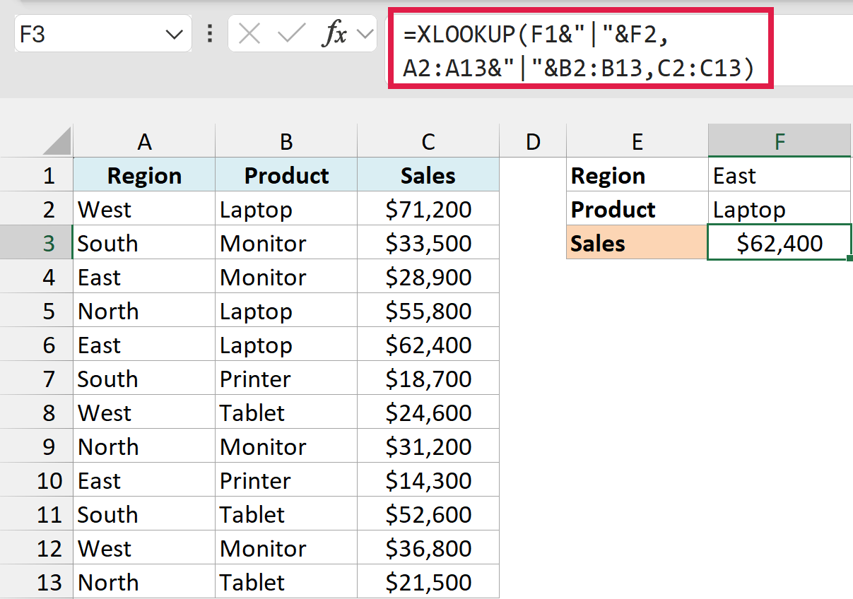
=XLOOKUP(F1&"|"&F2,A2:A13&"|"&B2:B13,C2:C13)
How does this formula work?
F1&"|"&F2 joins the two inputs into one lookup value, East|Laptop. A2:A13&"|"&B2:B13 does the same for every row, so you get a list like West|Laptop and South|Monitor.
XLOOKUP finds East|Laptop in that list, which is row 6, and returns $62,400.
You need the pipe character (|) in the middle because, without a separator, “AB” and “C” would join to the same text as “A” and “BC”. When that happens, the formula can return the wrong row.
This method only does exact matches, so you can’t use it for conditions like >. For those, use the boolean method covered earlier.
XLOOKUP with Two Criteria Using a Helper Column
This uses the same joining idea, but you keep the joined region and product (the key) in its own helper column, so you can see it right there in your data. Then the lookup itself is a plain XLOOKUP with one lookup value.
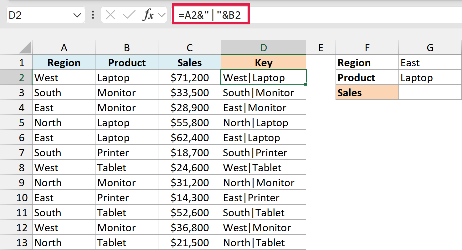
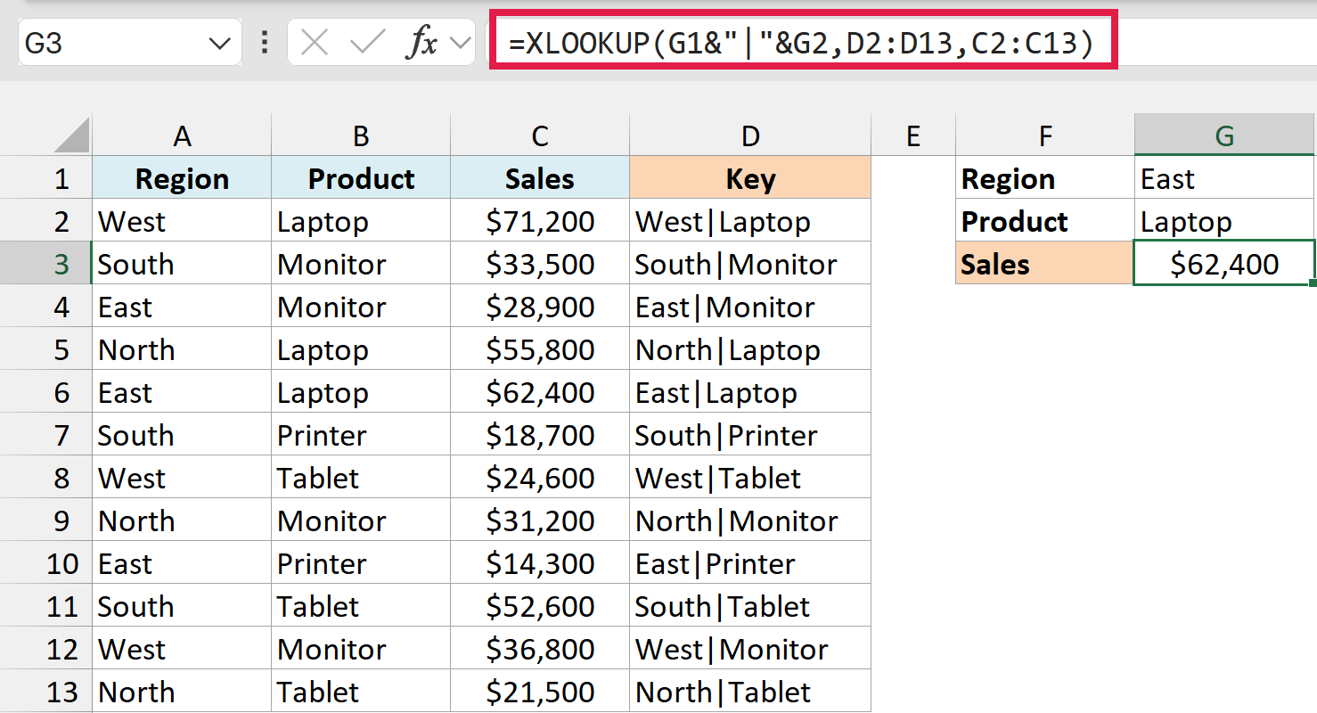
Below is the sales summary, and I want to build a key in column D and then get the sales in G3 for the region in G1 and the product in G2.
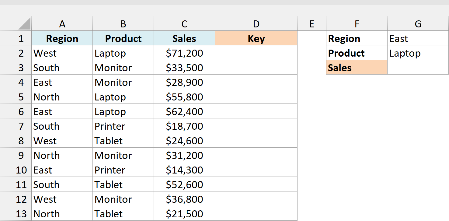
Enter the below formula in cell D2 and copy it down to D13:
=A2&"|"&B2
Now here is the formula that looks up the key:
=XLOOKUP(G1&"|"&G2,D2:D13,C2:C13)
How does this formula work?
G1&"|"&G2 builds the same key from the two inputs, East|Laptop. XLOOKUP finds it in column D, on row 6, and returns $62,400 from column C.
Since XLOOKUP can return a column to the left of the lookup column, the helper can sit at the end of your data. With VLOOKUP with multiple criteria, the helper has to be the first column of the lookup table.
The catch is that a new row needs its own key. If you convert your data to an Excel Table (Control + T), the key formula fills down by itself when you add a row, and the ranges in the lookup formula grow with it.
In this article, I showed you how to use XLOOKUP with multiple criteria using boolean logic, concatenation, and a helper column. I also covered three or more criteria, comparison conditions, OR logic, the latest match, and how to handle no match.
I hope you found this article helpful.
Other Excel Articles You May Also Like: