

If you have a list where the same value repeats, you may want every occurrence of that value to carry the same serial number, no matter where it shows up in the list.
A regular 1, 2, 3 fill won’t do this, because it gives every row a different number. But it’s simple to fix with a formula, and in this tutorial I’ll show you two easy ways to do it.
Let’s say you have a list of countries where the same country appears many times. You want every “India” to be numbered 1, every “USA” to be 2, and so on, so the number depends on the value and not the row it sits in.
The numbering follows the order in which each country first appears. The first country in the list becomes 1, the next new country becomes 2, and any repeat of a country you’ve already seen gets that country’s original number.
I’ll cover two ways to do this. The first uses XLOOKUP and a small lookup table. The second uses a single formula that updates on its own as your list changes.
Method 1: Assign the Same Serial Number Using XLOOKUP
XLOOKUP is the cleanest option here. It works well when your list of values doesn’t change very often.
Below I have a list of countries in column A, and I want to fill column B with a serial number for each one. Every country should always get the same number wherever it appears.
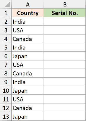
The idea is simple. First, build a small table that lists each country once with the number you want to give it. Then use XLOOKUP to pull that number next to every country in the main list.
Start by creating the lookup table. List each country a single time, then type a serial number beside it (1, 2, 3, 4).
To get the list of unique countries quickly, use the UNIQUE function in Excel 365, or run Data > Remove Duplicates on a copy of the column in older versions.
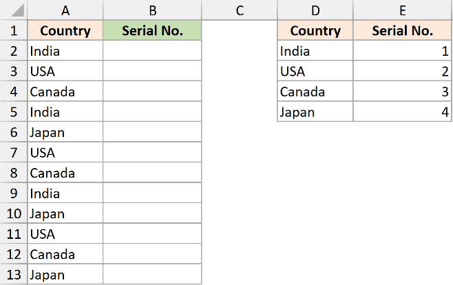
With the lookup table ready in D2:E5, use this XLOOKUP formula in cell B2:
=XLOOKUP(A2:A13,D2:D5,E2:E5)
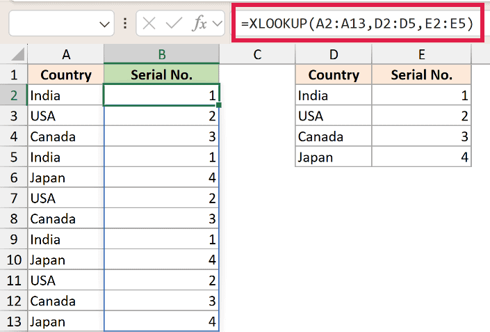
This looks up each country from the main list (A2:A13) in the country column of the lookup table (D2:D5) and returns the matching serial number from E2:E5. The single formula spills down the whole column on its own, so there’s nothing to copy.
XLOOKUP is available in Excel 365 and Excel 2021. One nice thing about it is that the lookup column and the result column can be in any order, so you’re not forced to keep the numbers to the right of the country names.
Pro Tip: On older versions without XLOOKUP, use VLOOKUP instead. Put =VLOOKUP(A2,$D$2:$E$5,2,FALSE) in the top cell and copy it down. With VLOOKUP the country names have to sit in the leftmost column of the lookup table.
Method 2: Assign the Same Serial Number with a Dynamic Formula
The VLOOKUP method works, but you have to build and maintain the lookup table by hand. If you add a new country later, you have to update that table too. This method uses a single formula that handles everything on its own.
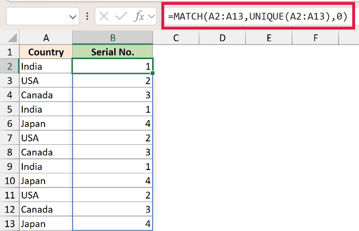
Below I have the same list of countries in column A, and I want the matching serial numbers in column B.
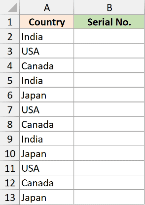
If you have Excel 365, this one formula in cell B2 does the whole job:
=MATCH(A2:A13,UNIQUE(A2:A13),0)
How this formula works:
- UNIQUE(A2:A13) gives you a list of each country once, in the order they first appear (India, USA, Canada, Japan).
- MATCH then looks up each country from the main list in that unique list and returns its position. India is first in the unique list, so every India returns 1. USA is second, so every USA returns 2, and so on.
Because MATCH is fed the whole column A2:A13, the result spills down the column on its own. Add or remove a country and the numbers update instantly, with no lookup table to maintain.
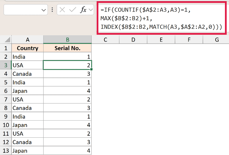
If you don’t have Excel 365, you can still do this with a slightly longer formula that works in older versions too.
Type 1 in cell B2. Then enter this formula in cell B3 and copy it down to the bottom of your list:
=IF(COUNTIF($A$2:A3,A3)=1,MAX($B$2:B2)+1,INDEX($B$2:B2,MATCH(A3,$A$2:A2,0)))
How this formula works:
- COUNTIF($A$2:A3,A3)=1 checks whether the country in the current row is showing up for the first time.
- If it’s the first time, MAX($B$2:B2)+1 finds the highest serial number used so far and adds 1 to it, giving that country a new number.
- If the country has appeared before, INDEX and MATCH go back to its first appearance and return the same number it got there.
It brings together the IF, COUNTIF, MAX, INDEX, and MATCH functions, but you only have to type it once and copy it down.
Tips and Common Mistakes
- The serial number follows the order in which each value first appears, not alphabetical order. If you’d rather number them alphabetically, sort your lookup list (Method 1) alphabetically before you assign the numbers.
- Keep your data in a single unbroken list. A blank row in the middle can throw off the count in the dynamic formula.
- If you just want plain 1, 2, 3 serial numbers down a column and don’t need to match duplicates, that’s a different (and simpler) task. See how to number rows in Excel for the quickest ways to do that.
And that’s how you give duplicate values the same serial number in Excel.
If your list rarely changes, the XLOOKUP method is quick to set up. If it changes often, the dynamic formula saves you from rebuilding a lookup table every time.
Other Excel Articles You May Also Like:

Need a serial number
I need a serial number