

If you want to put the logical value FALSE into a cell or a formula, the FALSE function is the simplest way to do it. You just type =FALSE() and you get back FALSE.
It takes no arguments and always returns the same thing, so it does not spill or work with ranges the way most functions do.
In this article I’ll show you how the FALSE function works and where it actually comes in handy, from IF formulas to comparisons and exact-match lookups.
FALSE Function Syntax
Here is the syntax of the FALSE function:
=FALSE()
The FALSE function has no arguments. You just add the opening and closing parentheses and it returns the logical value FALSE.
You can also type the word FALSE straight into a cell or a formula without the parentheses, and Excel reads it as the same logical value. The function exists mainly for compatibility with other spreadsheet programs, which is why it feels so bare.
FALSE works in Excel for Microsoft 365, Excel 2024, 2021, 2019, 2016, and Excel on the web, so you can use it just about anywhere.
When to Use the FALSE Function
Use the FALSE function when you need to:
- Put a clean logical FALSE into a cell or a formula
- Return FALSE as the result of a logical test (a comparison, or an AND / OR check)
- Set the value_if_false part of an IF formula
- Force an exact match in a lookup, like the last argument of VLOOKUP
- Feed a zero into a calculation, since Excel treats FALSE as 0
Let me show you a few practical examples of how this works.
Example 1: Return FALSE With the FALSE Function
Let’s start with the simplest case.
You don’t need any data for this one. On a blank worksheet, click any empty cell where you want the result to appear.
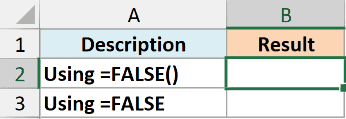
I want to return the logical value FALSE in that cell.
Here is the formula:
=FALSE()
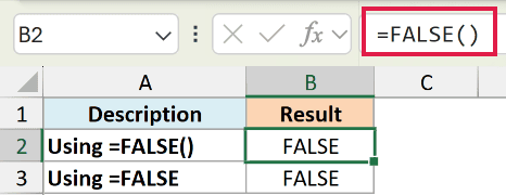
The cell now shows FALSE. There is nothing to configure, since the function takes no arguments and always returns the same value.
You can also skip the parentheses and just type the word FALSE with an equals sign in front.
=FALSE
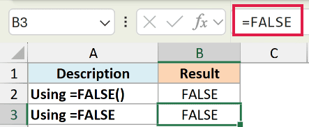
This gives you the exact same result. Excel reads FALSE as the logical value whether or not you add the parentheses.
Pro Tip: You can even type FALSE without the equals sign, and Excel still stores it as the logical value FALSE, not as text. So =FALSE(), =FALSE, and a plain FALSE all land in the same place.
Example 2: Get a TRUE or FALSE Result When Comparing Two Columns
Here’s a common one. FALSE shows up on its own whenever a comparison you write turns out to be untrue.
Below I have a stock check with the item in column A, the system count in column B, and the physical count in column C. I want to flag the rows where the two counts don’t match.
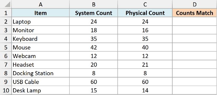
I want a TRUE where the counts agree and a FALSE where they differ.
Here is the formula:
=B2=C2
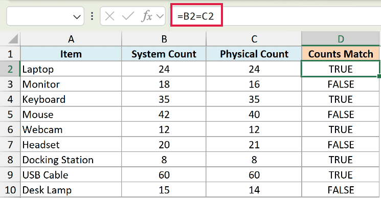
For each row, Excel checks whether the system count equals the physical count. When they match you get TRUE, and when they don’t you get FALSE.
Copy this down the column and every FALSE points you straight to a row where the two counts are out of sync. You didn’t type FALSE anywhere, the comparison produced it for you.
Example 3: Use FALSE as the Result in an IF Formula
Now let’s use FALSE inside a formula on purpose. The IF function takes a value to return when the test is true and another for when it’s false, and FALSE is a handy thing to put in that second slot.
Below I have a sales sheet with the rep in column A, their sales in column B, and the target in column C. I want to work out the commission, but only for reps who hit their target.
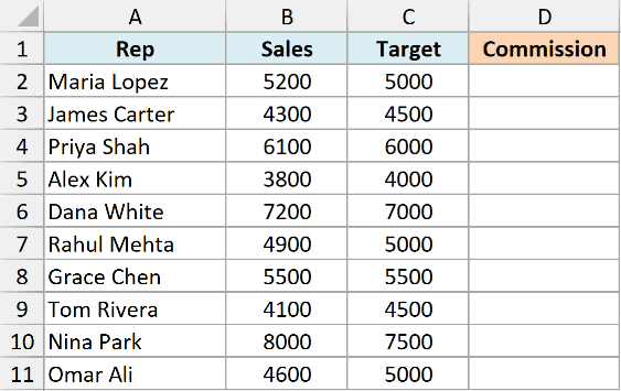
I want to show a 10% commission when sales reach the target, and FALSE when they don’t.
Here is the formula:
=IF(B2>=C2,B2*0.1,FALSE())
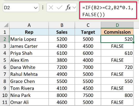
If the rep’s sales are at or above target, the formula returns the commission. If not, it returns FALSE, which reads as a clear “no commission” flag you can filter on or use in a later calculation.
Pro Tip: If you leave the value_if_false argument out of an IF formula completely, Excel returns FALSE by default. So =IF(B2>=C2,B2*0.1) gives the same result as spelling out FALSE() at the end.
Example 4: Return FALSE From AND and OR Tests
The AND and OR functions also hand you a FALSE when their conditions aren’t met, so they’re a natural fit here.
Below I have an order list with the order amount in column B and whether the customer is a member in column C. I want to check who qualifies for free shipping, which needs an order of at least 50 and a member.
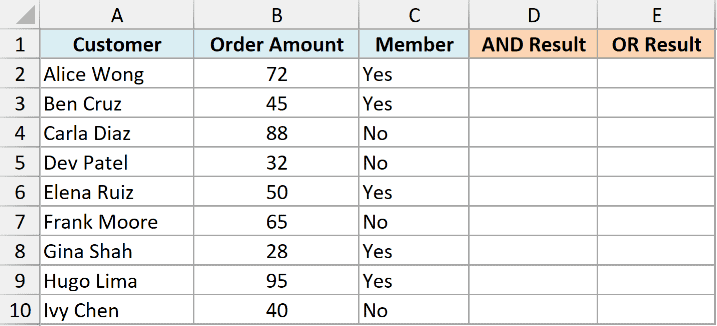
I want a TRUE only when both conditions are met, and a FALSE otherwise.
Here is the formula:
=AND(B2>=50,C2="Yes")
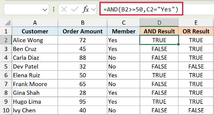
AND returns TRUE only when every condition is true. The moment one part fails, like an order under 50 or a non-member, it returns FALSE.
OR works the other way. It returns TRUE if at least one condition is met, and only returns FALSE when they all fail.
=OR(B2>=50,C2="Yes")
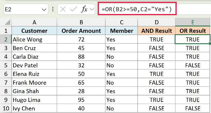
Here a row returns FALSE only when the order is under 50 and the customer is not a member. If either one is true, you get TRUE instead.
Example 5: Treat FALSE as Zero in a Calculation
This one trips people up in a good way. Excel stores FALSE as the number 0 (and TRUE as 1), so you can pull a TRUE/FALSE column straight into math.
Below I have a task list with the task in column A and a Completed column in column B that holds TRUE or FALSE. I want to count how many tasks are done.
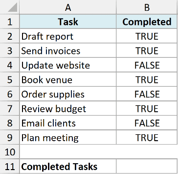
I want a single number that totals up all the TRUE values in the Completed column.
Here is the formula:
=SUMPRODUCT(--(B2:B9))
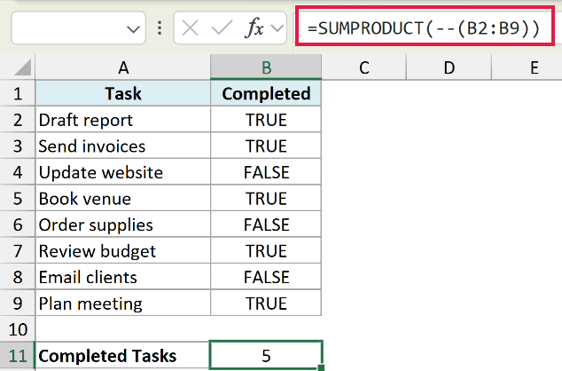
The double minus (--) forces each TRUE to 1 and each FALSE to 0, and SUMPRODUCT adds them up. So the result is simply the count of completed tasks.
This is the same coercion at work in small formulas too. =FALSE*1 returns 0 and =FALSE+1 returns 1, because FALSE is just 0 wearing a logical label.
Example 6: Use FALSE for an Exact Match in VLOOKUP
Finally, here’s where a lot of people meet FALSE without even thinking of it as a function. The VLOOKUP function takes FALSE as its last argument to force an exact match.
Below I have a product table with the product ID in column A, the name in column B, and the price in column C. I want to look up the price for a specific ID typed in cell E2.
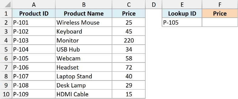
I want the exact price for the ID in E2, not the closest one.
Here is the formula:
=VLOOKUP(E2,A2:C10,3,FALSE)
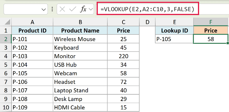
The FALSE at the end tells VLOOKUP to return a value only when it finds an exact match for the ID. Leave it out (or use TRUE) and VLOOKUP does an approximate match, which can quietly hand you the wrong price.
Pro Tip: If you’re on Excel 365 or 2021, the XLOOKUP function does an exact match by default, so you don’t need to remember the FALSE argument at all. FALSE is only there for the older lookups like VLOOKUP and HLOOKUP.
Tips and Common Mistakes
A few things worth keeping in mind with the FALSE function:
- FALSE() and FALSE are the same thing. Typing the function, typing =FALSE, or even typing the plain word FALSE all give you the same logical value. The function version exists mainly for compatibility with other spreadsheet programs.
- You rarely need to type FALSE yourself. A comparison like =B2=C2 or a test like =AND(…) already returns TRUE or FALSE on its own. Wrapping that in =IF(B2=C2,TRUE,FALSE) just adds length without changing the answer.
- FALSE is a logical value, not the text “FALSE”. If a cell actually holds the word FALSE as text (say, after an import), it won’t behave as 0 in math and comparisons can miss it. Check with the ISLOGICAL function if you’re unsure.
- FALSE equals 0 in calculations. This is genuinely useful for counting or summing flags, but it also means a stray FALSE in a range you’re adding contributes 0, not an error.
- Need to flip a result? To turn a TRUE into FALSE (or the other way around), wrap it in the NOT function, which reverses any logical value.
- The FALSE function takes no arguments and won’t spill. It returns one value per call, so there’s nothing to feed it a range with. To get a whole column of FALSE results, you rely on the comparison or logical test producing them, as in the examples above.
Wrapping Up
The FALSE function is about as simple as Excel functions get. It returns the logical value FALSE, takes no arguments, and mostly shows up as the result of a comparison, inside an IF, or as the exact-match switch in a lookup.
Once you see FALSE as just a labeled 0 that answers “is this true?”, it stops being mysterious and starts being useful.
I hope you found this tutorial helpful.
Other Excel Articles You May Also Like:
