

The FVSCHEDULE function in Excel tells you what an amount grows to when the interest rate changes from one period to the next. You give it a starting amount and a list of rates, and it applies them one after the other.
That makes it handy whenever a single fixed rate doesn’t match reality, like a savings account whose rate moves every year or a salary that gets a different raise each time.
In this article, I’ll show you how FVSCHEDULE works with seven examples, from a simple savings balance to stacked discounts, yearly returns, and a projection up to a year you pick.
Follow along with the example file
FVSCHEDULE Function Examples.xlsx
FVSCHEDULE Function Syntax
Here is the syntax of the FVSCHEDULE function:
=FVSCHEDULE(principal, schedule)
- principal – Required. The starting amount, which is the value you have today.
- schedule – Required. The list of rates to apply, in order. This can be a range of cells or a list of rates typed inside curly braces.
FVSCHEDULE applies each rate to the amount it got from the previous rate. With 5% and then 4% on $1,000, it first grows $1,000 to $1,050, and then grows $1,050 by 4%, which gives $1,092.
The rates in the schedule need to be decimals (0.05) or percentages (5%). If you type a plain 5, FVSCHEDULE reads it as 500%, and the result shoots way up.
The FVSCHEDULE function works in Excel 365, 2024, 2021, 2019, and 2016, and in Excel for Mac (365, 2024, and 2021).
When to Use the FVSCHEDULE Function
Use this function when you need to:
- Find what savings or an investment will grow to when the interest rate changes every year.
- Work out a salary, price, or fee after a series of different percentage increases.
- Apply several discounts one after another to get the final price.
- Turn a list of yearly returns into a total return or an average annual return.
- Project a value forward using a planned growth rate for each year.
Let me show you a few practical examples of how to use the FVSCHEDULE function.
Example 1: Future Value With a Different Rate Each Year
Let’s start with the job FVSCHEDULE was made for.
Below I have the interest rate a savings account paid each year from 2019 to 2026, and I want the balance at the end of 2026 in cell E3, starting from the $12,000 in cell E2.
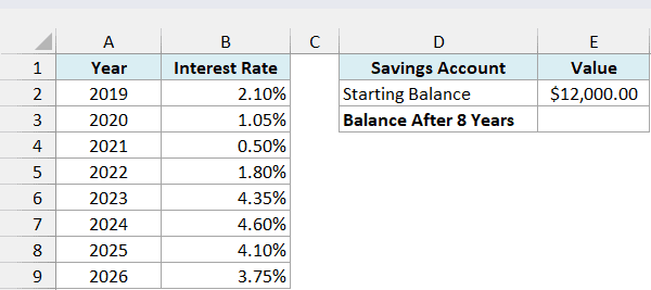
Here is the formula:
=FVSCHEDULE(E2,B2:B9)
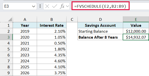
This gives $14,932.07, so the $12,000 earned $2,932.07 in interest over the eight years.
In the above formula, E2 is the principal and B2:B9 is the schedule. FVSCHEDULE grows the $12,000 by 2.10% for 2019, then grows that new balance by 1.05% for 2020, and keeps going until it has applied the 3.75% for 2026.
Important: Select only the cells with the rates. If your schedule range includes the header in B1, FVSCHEDULE returns a #VALUE! error, because the text “Interest Rate” isn’t a number.
If the rate stayed the same every year, you wouldn’t need a list of rates at all. The FV function handles that case with a single rate.
Example 2: Calculate a Salary After Yearly Raises
Interest isn’t the only thing that compounds. Raises work the same way, and this example also shows what happens when a year has no rate at all.
Below I have the raise someone got each year from 2020 to 2026, with no raise in 2022, and I want their current salary in cell E3, starting from the $58,000 in cell E2.
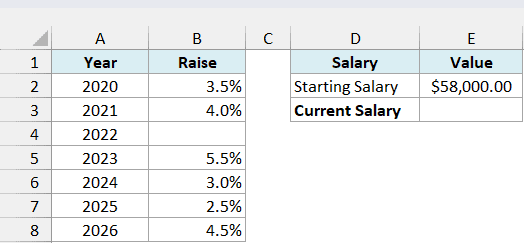
Here is the formula:
=FVSCHEDULE(E2,B2:B8)
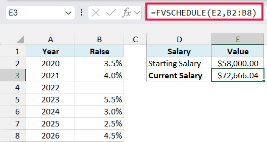
This returns $72,666.04.
The cell for 2022 (B4) is blank. FVSCHEDULE treats a blank cell as 0%, so the salary stays the same that year, and the calculation carries on with the 2023 raise.
The raises add up to 23%, but the salary went up by about 25.3%. That’s because each raise is applied to the salary after the previous raise, not to the original $58,000.
Important: For a year with no raise, leave the cell blank or enter 0%. If you type text like “None” or “Freeze”, FVSCHEDULE returns a #VALUE! error.
Example 3: Enter the Rates Directly in the FVSCHEDULE Formula
If you only want a quick estimate, you don’t need to put the rates in cells.
Below I have a monthly grocery bill of $650 in cell B2, and I want to estimate in cell B3 what it will be after three years of 3.2%, 2.7%, and 3.5% price increases.
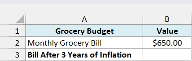
Here is the formula:
=FVSCHEDULE(B2,{0.032,0.027,0.035})
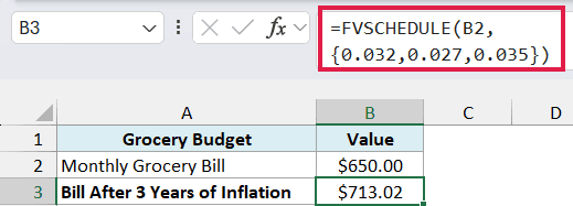
This gives $713.02.
The curly braces create an array constant, which is a list of values typed right inside the formula. FVSCHEDULE reads it the same way it reads a range of cells, with the rates separated by commas.
This is fine for a one-off estimate. When the rates might change, put them in cells instead (like in the first two examples), so you can update them without editing the formula.
Example 4: Apply Stacked Discounts to a List of Prices
FVSCHEDULE works with negative rates too, which turns it into a quick way to apply one discount after another.
Below I have a list of products with their prices, along with a 25% holiday sale and a 10% coupon in F2:F3, and I want the final sale price of every product in column C.
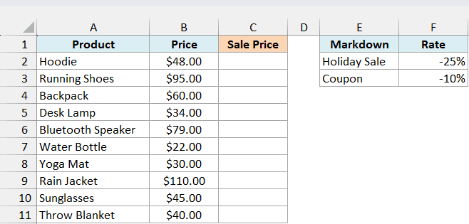
Here is the formula:
=FVSCHEDULE(+B2:B11,F2:F3)
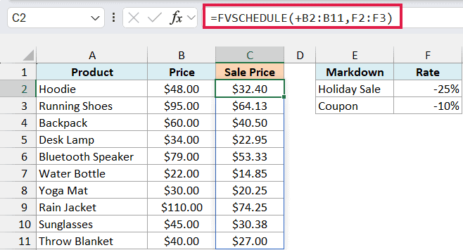
You enter this one formula in cell C2, and it fills the sale price for all ten products. The $48 hoodie comes down to $32.40.
How this formula works:
- F2:F3 holds the two discounts as negative rates (-25% and -10%). A negative rate shrinks the amount instead of growing it, so the hoodie works out as $48 × 0.75 × 0.90.
- +B2:B11 is the list of prices. The plus sign in front matters, because FVSCHEDULE doesn’t accept a range of cells as the principal and returns a #VALUE! error for =FVSCHEDULE(B2:B11,F2:F3).
- With the plus sign, Excel turns the range into a list of values, runs FVSCHEDULE once for each price, and spills the ten results into C2:C11.
Notice that the two discounts don’t add up to 35% off. The coupon applies to the already reduced price, so the total discount is 32.5%, and the hoodie ends at 67.5% of its original price.
For the spill to work, C3:C11 must be empty. If anything is already in those cells, you get a #SPILL! error instead.
If you are using Excel 2019 or earlier, enter the below formula in cell C2 and then copy it down to C11:
=FVSCHEDULE(B2,$F$2:$F$3)
The dollar signs lock the discount cells, so every row keeps using F2:F3 when you copy the formula down.
Example 5: Show the Value Year by Year
FVSCHEDULE gives you one final number, but sometimes you want to see the value at the end of every year along the way.
Below I have the yearly tuition increase at a college from 2019 to 2026, and I want the tuition for each year in column C, starting from the 2018 tuition of $9,800 in cell F2.
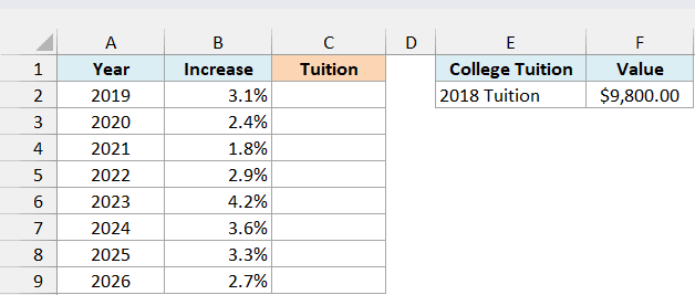
Enter the below formula in cell C2 and then copy it down to C9:
=FVSCHEDULE($F$2,$B$2:B2)
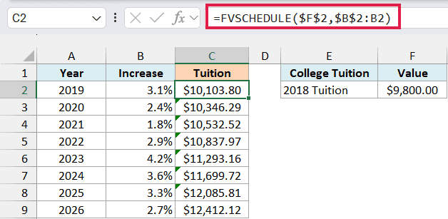
This shows the tuition going from $10,103.80 in 2019 to $12,412.12 in 2026.
What makes this work is the schedule range $B$2:B2. Its start is locked and its end isn’t, so the range grows as you copy the formula down.
In C3 it becomes $B$2:B3 (the 2019 and 2020 increases), and in C9 it covers all eight years.
You may see small green triangles in C3:C8. Excel flags these cells because each range stops before the rest of the increases in column B, which is exactly what we want here, so you can ignore them.
This can’t be one spilling formula like in Example 4. There, each price was its own principal and got its own result.
Here there’s only one principal, and FVSCHEDULE turns a whole schedule into a single value. So each year needs its own formula, with a schedule that ends at that year.
Example 6: Find the Total Return and Average Annual Return
This one is useful if you track the yearly returns of an investment.
Below I have the yearly returns of a retirement fund from 2019 to 2026, including two years with losses, and I want the total return and the average annual return in column E.
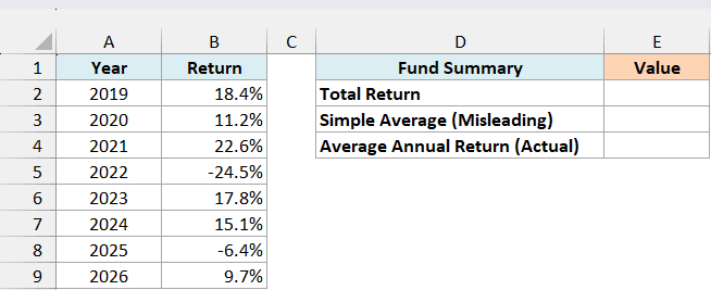
Here is the formula for the total return:
=FVSCHEDULE(1,B2:B9)-1
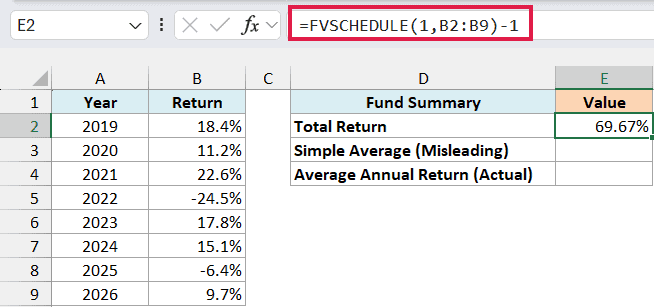
This returns 69.67%.
Using 1 as the principal is the trick here. FVSCHEDULE grows 1 through all eight returns and gives about 1.6967, and subtracting 1 leaves just the growth, so every $1 in the fund at the start of 2019 became about $1.70.
Now for the average return per year. You might be tempted to use the AVERAGE function on these returns, so here is that formula:
=AVERAGE(B2:B9)
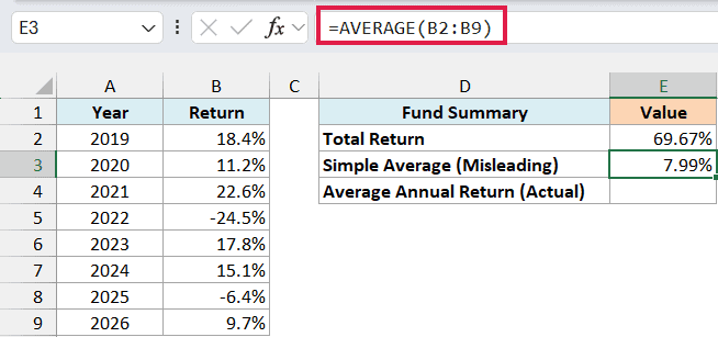
This gives 7.99%, which is too high. If the fund had really grown 7.99% every year, it would be up about 84.9% after eight years, not 69.67%.
The simple average misses that a loss shrinks the amount the later gains build on. After the 24.5% drop in 2022, the fund needed a gain of about 32.5% just to get back to where it was.
Here is the formula for the real average annual return:
=FVSCHEDULE(1,B2:B9)^(1/ROWS(B2:B9))-1
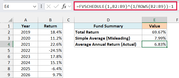
This returns 6.83%.
The formula takes the total growth from FVSCHEDULE, finds its eighth root (ROWS(B2:B9) counts the eight years), and subtracts 1. The result is the one steady yearly rate that ends at the same 69.67% total.
This is the same idea as the compound annual growth rate (CAGR), just worked out from yearly returns instead of a start and end value.
Pro Tip: The RRI function gives the same 6.83%. Give it the number of years, a starting value of 1, and the FVSCHEDULE result: =RRI(ROWS(B2:B9),1,FVSCHEDULE(1,B2:B9)).
Example 7: Project a Value Up to a Chosen Year
Let’s step it up and combine FVSCHEDULE with the FILTER function.
Below I have a bakery’s planned sales growth for each year from 2026 to 2033, its 2025 sales of $240,000 in cell E2, and a year in cell E3, and I want the projected sales for that year in cell E4.
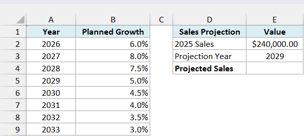
Here is the formula:
=FVSCHEDULE(E2,FILTER(B2:B9,A2:A9<=E3))
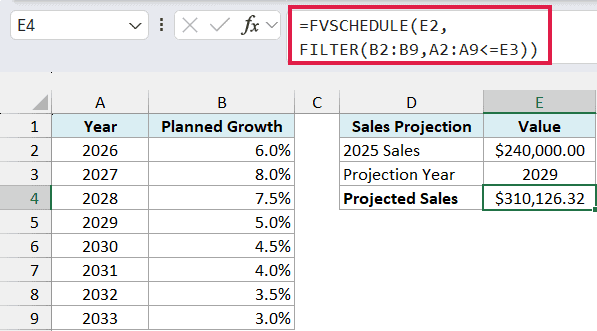
With 2029 in E3, this returns $310,126.32.
How this formula works:
- FILTER(B2:B9,A2:A9<=E3) keeps only the growth rates for the years up to and including 2029, which are 6%, 8%, 7.5%, and 5%.
- FVSCHEDULE then applies those four rates to the $240,000.
Change the year in E3 to 2031, and the formula picks up two more rates without any other edits. If you enter a year before 2026, the FILTER function finds no rates and the formula returns a #CALC! error.
A year after 2033 doesn’t give an error. The formula simply uses all eight rates, so make sure the year you enter falls inside your plan.
The FILTER function is available in Excel 365 and Excel 2021 or later. If you are using Excel 2019 or earlier, enter the below formula in cell E4 instead:
=FVSCHEDULE(E2,B2:INDEX(B2:B9,MATCH(E3,A2:A9,0)))
Here, the MATCH function finds the position of the chosen year, and the INDEX function turns it into a reference to that year’s rate. So B2:INDEX(…) becomes B2:B5 for 2029, and FVSCHEDULE uses the rates in that range.
This version needs the year to be in column A. For a year before 2026 or after 2033, the MATCH function can’t find it, and the formula returns a #N/A error.
So these are seven ways to use the FVSCHEDULE function in Excel, from a savings balance with changing rates to stacked discounts and a projection up to any year.
Whatever the rates stand for, FVSCHEDULE applies each one on top of the result of the one before. I hope you found this tutorial useful.
Other Excel Articles You May Also Like:
