
Watch Video – How to Insert Picture into a Cell in Excel
A few days ago, I was working with a data set that included a list of companies in Excel along with their logos.
I wanted to place the logo of each company in the cell adjacent to its name and lock it in such a way that when I resize the cell, the logo should resize as well.
I also wanted the logos to get filtered when I filter the name of the companies.
Wishful Thinking? Not Really.
You can easily insert a picture into a cell in Excel in a way that when you move, resize, and/or filter the cell, the picture also moves/resizes/filters.
Below is an example where the logos of some popular companies are inserted in the adjacent column, and when the cells are filtered, the logos also get filtered with the cells.
This could also be useful if you’re working with products/SKUs and their images.
When you insert an image in Excel, it not linked to the cells and would not move, filter, hide, and resize with cells.
In this tutorial, I will show you how to:
- Insert a Picture Into a Cell in Excel.
- Lock the Picture in the cell so that it moves, resizes, and filters with the cells.
Insert Picture into a Cell in Excel
Here are the steps to insert a picture into a cell in Excel:
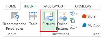
- Go to the Insert tab.
- Click on the Pictures option (it’s in the illustrations group).

- In the ‘Insert Picture’ dialog box, locate the pictures that you want to insert into a cell in Excel.

- Click on the Insert button.
- Re-size the picture/image so that it can fit perfectly within the cell.

- Place the picture in the cell.
- A cool way to do this is to first press the ALT key and then move the picture with the mouse. It will snap and arrange itself with the border of the cell as soon it comes close to it.

- A cool way to do this is to first press the ALT key and then move the picture with the mouse. It will snap and arrange itself with the border of the cell as soon it comes close to it.
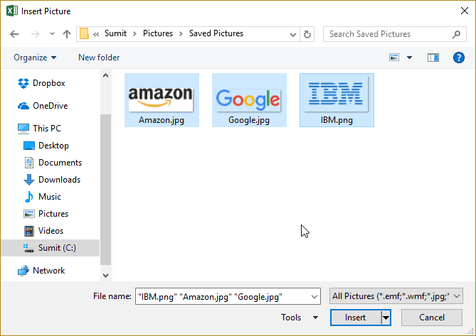


If you have multiple images, you can select and insert all the images at once (as shown in step 4).
You can also resize images by selecting it and dragging the edges. In the case of logos or product images, you may want to keep the aspect ratio of the image intact. To keep the aspect ratio intact, use the corners of an image to resize it.
When you place an image within a cell using the steps above, it will not stick with the cell in case you resize, filter, or hide the cells. If you want the image to stick to the cell, you need to lock the image to the cell it’s placed n.
To do this, you need to follow the additional steps as shown in the section below.
Also read: How to Start a New Line in Excel Cell
Lock the Picture with the Cell in Excel
Once you have inserted the image into the workbook, resized it ti fit within a cell, and placed it in the cell, you need to lock it to make sure it moves, filters, and hides with the cell.
Here are the steps to lock a picture in a cell:
- Right-click on the picture and select Format Picture.

- In the Format Picture pane, select Size & Properties and with the options in Properties, select ‘Move and size with cells’.


That’s It!
Now you can move cells, filter it, or hide it, and the picture will also move/filter/hide.
Try it yourself.. Download the Example File

This could be a useful trick when you have a list of products with their images, and you want to filter certain categories of products along with their images.
You can also use this trick while creating Excel Dashboards.
You May Also Like the Following Excel Tutorials:


47 thoughts on “How to Insert Picture Into a Cell in Excel (a Step-by-Step Tutorial)”
It makes the job easy
Tanx
Thank you very much for sharing this. Simple and easy to follow.
Thank you for sharing. Love this excel tip.
Is there a way to flatten/minimize the size of the images so that the file does not get so big? My document has multiple tabs, and lots of other data besides the images, so I’d like to minimize the image but keep it from getting pixelated.
Thanks so much for that – so simple! I regard myself as pretty useful with Excel but could never find how to do that!
Thank you! I was looking for a way to lock an image in a cell so that it wasn’t floating around!
Thank you!! That was super helpful 🙂
Thank you very much. This is great.
Is there a way to format a whole column of images at once? I want them all to filter without having to right click on each one
Hi Trevor, you can select all objects (ie pictures) at once by clicking on Find & Select, Go To Special and then Objects. This will show all objects as selected. Then you can change the format of them all at the same time
In which version of excel you do this technique, because in my version this did not work
Thank you! I used to day – big help!
amazing, I can’t wait to use it, thanks
Thanks Excellent solution , keep posting new features
Wonderful! Rarely did I come across such illustrative and clear guidelines, thanks.
Hi
Can we do the same with excel vba?
I mean macro?
Excellent
amazing! my hero
from Bibendum wine
Thanks, it helped me a lot
Thank you very much!
Thank you so much, I know it must been a way for it a long time ago now I decided to search for it.
I want to insert / show a picture if i enter a date in another cell. Please hel[p
Oh sorry, I wrote my first call in German. Here is it in English:
I did all, as mentioned above, but for sure with some differences due to the Excel 2016 Version I use.
Shortly:
a. I included 2 pictures by means of the Insert button at the very up menu row. Include Picture. Then
b. I clicked right mouse and click “Size and properties” and then activated the upper button: “depending from cell position and size”.
c. When I try to insert the picture into another cell, e.g. with =$A$1 only a 0 appears. The picture is NOT shown.
What is wrong???
Thanks in advance for helpful remarks.
Udo
This is also my problem. I’m not sure how to reference the photo/image so that it can be pulled into a different tab/workbook using a formula.
Ich habe das alles gemacht. In Excel 2016 habe ich die Bilder eingefügt mit dem Einfügen/Bilder Befehl (oberste Menüleiste), dann über rechte Maustaste “Größe und Eigenschaften” gewählt und dann”von Zellposition und Größe abhängig” angeklickt.
Wenn ich jetzt z.B. mit =$A§1 das Bild anspreche, erscheint nur eine Null 0, die Zelle ist ja auch leer. Wie kann ich das Bild sichtbar kriegen???
Danke
Udo
I like excell info
Amazing. Thank you very much for sharing!
Thanks Sumit. It was very self-explanatory. Detailed yet to the point. Was looking for something like this since long!
very useful THANKS
Thank you very much… good tutorial & Helpful.
Thanks. Knew it was possible, but didn’t remember where to find the settings for it.
It almost worked. I have a free add-in for flash cards that picks up on the cell contents to make the flash cards. It does not recognize that the cell with the graphic has contents. I fed this page back to the developer in case he can figure out a way.
Thanks Sumit!!!
Very usefull! Thanks
Hiya could this be useful with a large data set i.e 1500 images? I have an advanced filter macro that utilizes data off a seperate tab where i would like to insert the images, just concerned it will be very slow due to the amount of images and want to find out before trying to insert that many images if it will not work, cheers!
this does not work for large set of images. bug i guess
this is awesome. good explanation. thanks
I don’t see how this makes it “filterable”, locking the image into the cell was described in this tutorial, but it seems that I missed the filter portion of it.
Hey Chris.. When you insert a picture in a cell in Excel and set the property to Move and Size with cell, it will get filtered with it. For example, from the company list, if you filter all the companies with the name Amazon in it, the images would also get filtered with the text
I have done this, but after using the filters editing other fields and saving the sheat multiple copies I realized, that the images got multiplacated somehow, and even overlaped. (Basically the image in N th row got copied to N+1th row even in cases, when there was an image there already.)
Do you know what the cause of this could be? And how to prevent it?
Thanks a lot for your help, I hope you know a solution to it
I’ve got the same bug. It happens on the first and last row in a filtered view. Very frustrating. Any idea on how to solve it?
Thanks for the tip
Simple indeed! You could also easily automate this process with Picture Manager for Excel add-in at http://doality.com
Thanks for sharing Artemy.. Will check it out!
Awesome tip. Thank you so much!
Glad you found this helpful!!