
In this tutorial, you’ll learn how to find the last occurrence of an item in a list using Excel formulas.
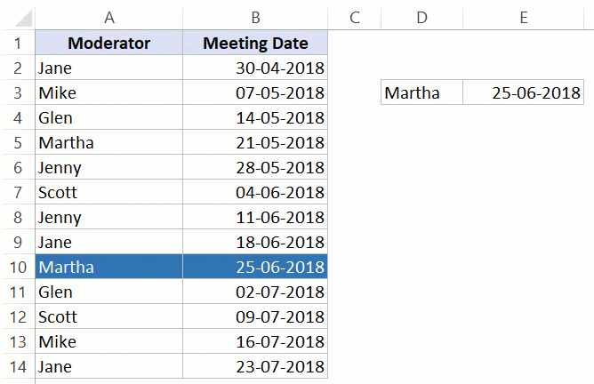
Recently, I was working on setting the agenda for a meeting.
I had a list in Excel where I had a list of people and the dates on which they acted as the ‘Meeting Chair’.
Since there was repetition in the list (which means that a person has been Meeting Chair multiple times), I also needed to know when was the last time a person acted as the ‘Meeting Chair’.
This was because I had to ensure someone who recently chaired was not assigned again.
So I decided to use some Excel Function magic to get this done.
Below is the final result where I am able to select a name from the drop-down and it gives me the date of the last occurrence of that name in the list.
If you have a good understanding of Excel Functions, you would know that there is no one Excel function that can do this.
But you are in the Formula Hack section, and here we make the magic happens.
In this tutorial, I’ll show you three ways to do this.
Find the Last Occurrence – Using MAX function
Credit to this technique goes to an article by Excel MVP Charley Kyd.
Here is the Excel formula that will return the last value from the list:
=INDEX($B$2:$B$14,SUMPRODUCT(MAX(ROW($A$2:$A$14)*($D$3=$A$2:$A$14))-1))
Here is how this formula works:
- The MAX function is used to find the row number of the last matching name. For example, if the name is Glen, it would return 11, as it’s in the 11 row. Since our list starts from second row onwards, 1 has been subtracted. So the position of the last occurrence of Glen is 10 on our list.
- SUMPRODUCT is used to ensure that you don’t have to use Control + Shift + Enter, as SUMPRODUCT can handle array formulas.
- INDEX function is now used to find the date for the last matching name.
Find the Last Occurrence – Using LOOKUP function
Here is another formula to do the same job:
=LOOKUP(2,1/($A$2:$A$14=$D$3),$B$2:$B$14)
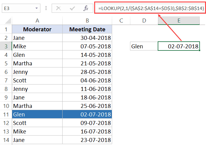
Here is how this formula works:
- The lookup value is 2 (you’ll see why.. keep reading)
- The lookup range is 1/($A$2:$A$14=$D$3) – This returns 1 when it finds the matching name and an error when it doesn’t. So you end up getting an array. For example, of the lookup value is Glen, the array would be {#DIV/0!;#DIV/0!;1;#DIV/0!;#DIV/0!;#DIV/0!;#DIV/0!;#DIV/0!;#DIV/0!;1;#DIV/0!;#DIV/0!;#DIV/0!}.
- The third argument ([result_vector]) is the range from which it gives the result, which are dates in this case.
The reason this formula works is that the LOOKUP function uses the approximate match technique. This means that if it can find the exact matching value, it would return that, but if it can not, it will scan the entire array till the end and return the next largest value which is lower than the lookup value.
In this case, the lookup value is 2, and in our array, we will only get 1’s or errors. So it scans the entire array and returns the position of the last 1 – which is the last matching value of the name.
Find the Last Occurrence – Using Custom Function (VBA)
Let me also show you another way of doing this.
We can create a custom function (also called User Defined Function) using VBA.
The benefit of creating a custom function is that it’s easy to use. You don’t have to worry about creating a complex formula every time, as most of the work happens in the VBA backend.
I have created a simple formula (which is a lot like VLOOKUP formula).
To create a custom function, you need to have the VBA code in the VB Editor. I will give you the code and the steps to place it in the VB Editor in a while, but let me first show you how it works:
This is the formula that will give you the result:
=LastItemLookup($D$3,$A$2:$B$14,2)
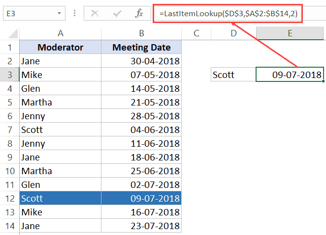
The formula takes three arguments:
- Lookup Value (this would be the name in cell D3)
- Lookup Range (this would be the range that has the names and dates – A2:B14)
- Column Number (this is the column from which we want the result)
Once you have created the formula and put the code in VB Editor, you can use it just like any other regular Excel worksheet functions.
Here is the code for the formula:
'This is a code for a function that finds the last occurrence of a lookup value and returns the corresponding value from the specified column
'Code created by Sumit Bansal (https://trumpexcel.com)
Function LastItemLookup(Lookupvalue As String, LookupRange As Range, ColumnNumber As Integer)
Dim i As Long
For i = LookupRange.Columns(1).Cells.Count To 1 Step -1
If Lookupvalue = LookupRange.Cells(i, 1) Then
LastItemLookup = LookupRange.Cells(i, ColumnNumber)
Exit Function
End If
Next i
End Function
Here are the steps to place this code in the VB Editor:
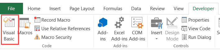
- Go to the Developer tab.
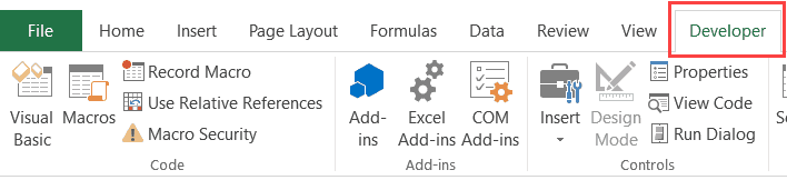
- Click on the Visual Basic option. This will open the VB editor in the backend.
- In the Project Explorer pane in the VB Editor, right-click on any object for the workbook in which you want to insert the code. If you don’t see Project Explorer go to the View tab and click on Project Explorer.
- Go to Insert and click on Module. This will insert a module object for your workbook.

- Copy and paste the code in the module window.

Now the formula would be available in all the worksheet of the workbook.
Note that you need to save the workbook in the .XLSM format as it has a macro in it. Also, if you want this formula to be available in all the workbooks you use, you can either save it to the Personal Macro Workbook or create an add-in from it.
You May Also Like the Following Excel Tutorials:


I have a table with one column that list the products ordered and at the end of the order the customer ID. I need to create two columns 1. cust id 2. product ordered.
Current table looks like this:
Apple
Cake
Coke
Cust:1 total=3
Tree
Apple
Plant
Cust:2 total=3
I want the table to look like this:
Prod Order ID
Apple Cust:1
Cake Cust:1
Coke Cust:1
Tree Cust:2
Apple Cust:2
Plant Cust:2
Any help would be appreciated. Excel or Access
On the custom function is there anything I need to change when range is a different sheet in the same workbook? I keep getting 0 as my result?
May I ask How to Find the Last Match in a Range with a Wildcard?
Thank you very much.
Thank you for this formula, however can you advise me how to include the INDIRECT function into my formula or to change the vba code so that when I copy this formula down to the next row the worksheet name changes to the next worksheet (my worksheet names are Unit 1, Unit 2 etc). I also have the worksheet names in column A that I can reference.
Unit No Name Amount Owing
Unit 1 Royce Smith -$20.00
Unit 2 Elly Howard $0.00
Unit 3 Sean Bright $0.00
Unit 4 Vicki Brown $0.00
=LastItemLookup($B2,’Unit 1′!$A$2:$J$1048576,10)
Thanks
Thank you!! This was exactly what I needed!!
Excellent ! Thanks a lot. It works like a charm. I even added some criteria, by adding them in the max formula [ MAX(ROW(range)*(range=value)*(range2=value2)…)-1 ]
PS : in google sheet, no need for the -1 at the end.
Thank you. The Lookup version did not work, probably because I have some blanks on my worksheet. However, the VBA version (with slight modification) works perfectly! Very helpful.
Hello!
Can you please tell me what formula to use for reading values (numbers) from the last 10 rows in a column? Periodically is added manually one row in the same column, so the formula would read each time the last 10 rows.
Thank you.
This is the exact function I was looking for. However, I want to be able to keep adding new entries below the original list, and every time I add a new entry below – excel will remember the values given to that last entry. For example: The items in column A are dates. Column B are names of participants (with drop down function). Column C values are weights for exercise number 1, and column D are weights for exercise number 2 that the participant completed on that date. Each day we add new entries – we don’t want to keep scrolling up the list find out what weight each participant completed in the previous session. We want excel to automatically fill this out in column C and D. We also want to be able to change this value (if participant progresses the weight), which will be remembered by excel in the next entry for that participant. I tried the methods above, but seems to not work..
Hello,
If I have a empty values, how can I find the last value different than empty?
Thanks
Thank you! this is very useful!
Thank You!!
I have a list of basketball scores by date, I want to find the last game a team played before today.
For example
column A has the home team (the team I want to find the most recent game played before today)
Column B has the away team
Column C has the score
I would like to be able to find the team in column A’s most recent game played before today and extract the their opponent (column b) and the score (column c).
Any help would be greatly appreciated. Thanks.
Is there an easy way to adjust the INDEX() function to return the FIRST occurrence, rather than the last? I tried switching the nested formula to MIN() instead of MAX(), but it doesn’t seem to work.
Hi Everyone,
I have a set of stock units transacted (ordered by date from old to new) and I want to find the Previous Quantity that was transacted. Here is a sample dataset:
Date Type Stock Qty PrevQty CumulativeQty
2016-01-03 Buy MSFT 100 0 100
2016-01-04 Buy GOOG 500 0 500
2016-01-05 Buy MSFT 100 100 200
2016-01-06 Sell MSFT 100 100 100
I am able to figure out CumulativeQty via SUMIFS but unable to do PrevQty. Any help would be highly appreciated.
Best,
-Ash
Works great, but I need it to search for partial text. In my case, I am searching for the next cell in column C after the last occurrence of “OK” in column H. I need to match all “OK – blahblah”.
=INDEX($C$60:$C$85,MATCH(1,MATCH($H$60:$H$85,H90,0),1)+1)
works, but requires exact text in H90.
Thanks for this, it was very helpful. IMO, one thing’s not very well explained. Put these formulas in cell E3, then fill in D3 with one of the values in column A, and E3 will tell you the date in column B that corresponds to the last occurance of that value.
use {} brackets in second case as well – {=MAX(IF(A:A=””,0,IF(A:A=0,1,0))*ROW(A:A),0)}
{=MAX(IF(A:A=”Apple”,1,0)*ROW(A:A),0)}
Where
First A:A is the range where you are looking for last occurrence (Can be any other range E.G. A4:B12).
Row(A:A) – relative multiplier (Can be any letter, but should be same first and last rows as in first range. E.G. if first range is A4:B12, row() should be row(A4:A12) or Row(A4:B12) or Row(C4:C12).
last A:A is the range
“Apple” can be anything you are looking for e.g. Number, Text, or cell reference (like D4)
P.S. If you are looking for 0, formula above will return last occurrence of 0 or blank cell. If you are looking exactly for 0 and not blank cell, use: =MAX(IF(A:A=””,0,IF(A:A=0,1,0))*ROW(A:A),0)
This same Match Formula works with Google Sheets as well! Very helpful. Thank you.
Hello, this is what I am looking for!
I looking to find the last “ok” in the row then give me the number the row next to it.
tried =LOOKUP(“ok”,G:G,F:F) gives not the last one but in the middle.
tried =OFFSET(INDEX(F:F,MATCH(“ok”,G:G)),0,0) gives the same result.
see attached picture I tried to get the balance next to the last “ok”
balance in row F
“ok” in row G
thanks in advance,
IMC
Hi Sumit
I tried this formula and it seems that your formula is returning the last date in some of the items and in other cases the date before the last occurrence. Am I doing something wrong in my setup?
When I change the first argument in the Match function from 1 to 2, everything seems to work fine. When the argument is 1, it seems to work for some but not for others.
{=+INDEX($J$2:$J$15,MATCH(1,MATCH($I$2:$I$15,L3,0),1))}
Feb 14 is the last occurrence for Steve and Jan 14th is the first occurrence. Is there something wrong in my set up
Steve 16-Jan-14 (Formula 2)
13-Feb-14 (Formula 1 – correct)
there are cases (depending on the sort order) where this will not return the last match – use this method instead – it will get you the last match no matter what: http://www.get-digital-help.com/2014/02/07/find-last-matching-value-in-an-unsorted-list/