How to Create a Drop Down List in Excel (Step-by-Step Guide)

If you want people to pick a value from a fixed list instead of typing it, a drop-down list is the way to do it. It takes only a few seconds to set up.

It’s useful when you’re getting someone to fill a form or a tracker, or when you’re building interactive Excel dashboards.

Drop-down lists are quite common on websites and apps, and they’re very intuitive for the user.

In this tutorial, I’ll show you how to create a drop-down list in Excel, make it update automatically when you add new items, and a few other useful things you can do with it.

How to Add a Drop Down List in Excel (Using a List of Cells)

Let’s start with the most common way, where the items for the drop-down are already in a list on your worksheet.

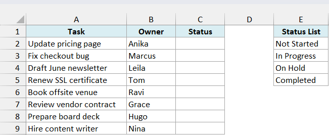
Below I have a task tracker with the tasks in column A and the owners in column B.

I want a drop-down in column C so the status of each task can be picked from the Status List in E2:E5.

Here are the steps to create the drop-down list:

1. Select the cells where you want the drop-down list (C2:C9 in this example).

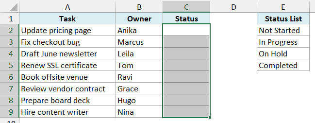
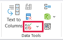
2. Click the Data tab, and then click Data Validation (it’s in the Data Tools group).

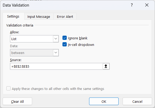
3. In the Data Validation dialog box, in the Settings tab, select List in the Allow drop-down.

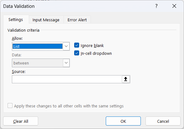
As soon as you select List, the Source field appears.

4. Click inside the Source field and select the cells E2:E5 with your mouse (or type =$E$2:$E$5).

5. Click OK.

This inserts a drop-down list in C2:C9. When you select any of these cells, you’ll see a small arrow. Click it and pick the status you want.

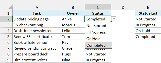
You can also open the drop-down with the keyboard shortcut ALT + Down Arrow.

Make sure the In-cell dropdown option in the dialog box is checked (it’s checked by default).

If it’s unchecked, the cell doesn’t show the arrow, but you can still only type the values from the list.

When you select the source cells with the mouse, Excel adds an absolute reference (=$E$2:$E$5 and not E2:E5).

If you type the reference instead, keep the dollar signs so every cell in C2:C9 points to the same list.

Pro Tip: In Microsoft 365, you can type a few letters in a drop-down cell and the list filters to show only the matching items. Handy when the list is long.

This matching works on text anywhere in the item, so typing “prog” finds In Progress. On older versions, you can build a searchable drop-down list instead.

Create a Drop Down List by Typing the Items

In the above example, the items for the drop-down came from cells. You can also type the items directly in the Source field.

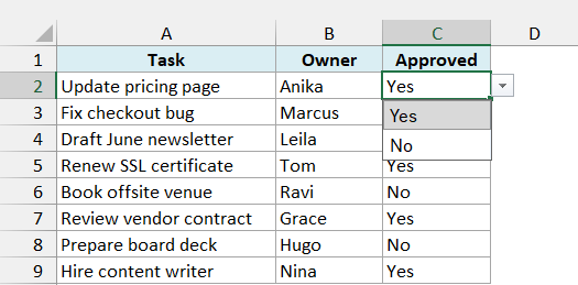
This works well for short lists that never change. For example, let’s say you want to show only two options, Yes and No, in the Approved column below.

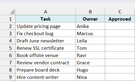
Here is how you can type the items in the Data Validation Source field:

1. Select the cells where you want the drop-down list (C2:C9 in this example).

2. Click the Data tab, and then click Data Validation.

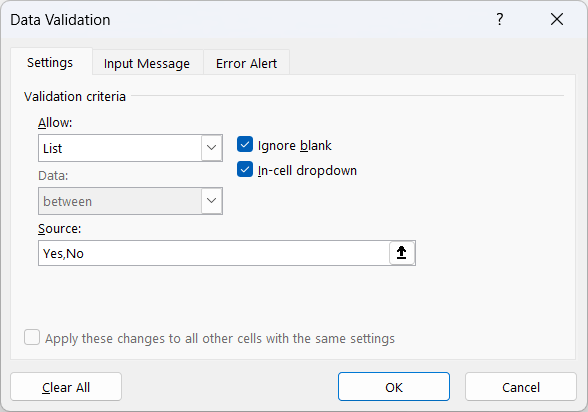
3. In the Settings tab, select List in the Allow drop-down.

4. In the Source field, type Yes,No

5. Click OK.

This creates a drop-down list in the selected cells. All the items you typed in the Source field, separated by a comma, show up on separate lines in the drop-down.

Important: If your Windows regional settings use a semicolon as the list separator (common in Europe), type Yes;No instead of Yes,No.

Since the items are hard-coded, you’ll have to open the Data Validation dialog box again whenever you want to change them.

Create a Dynamic Drop Down List Using an Excel Table

The drop-down in the first method uses a fixed range (E2:E5). If you add a new status, such as Cancelled, in cell E6, it won’t show up in the drop-down.

You’d have to go back and update the Source field every time the list changes. A better way is to turn the source list into an Excel Table.

Below I have the same task tracker, with the Status List in E1:E5.

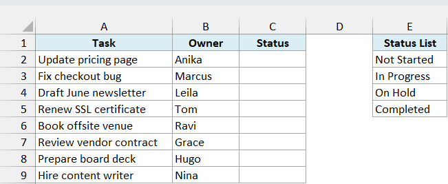
Here are the steps to create a drop-down list that updates automatically:

1. Select the Status List, including the header (E1:E5).

2. Press Ctrl + T (or go to Insert and click Table).

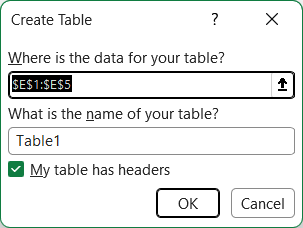
3. In the Create Table dialog box, make sure My table has headers is checked, and click OK.

4. Select C2:C9, click the Data tab, and then click Data Validation.

5. In the Settings tab, select List in the Allow drop-down.

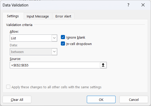
6. Click inside the Source field and select the items in the Table (E2:E5), without the header.

7. Click OK.

Now type Cancelled in cell E6, right below the Table. The Table expands to include it, and the drop-down’s source changes to =$E$2:$E$6 on its own.

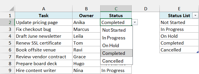
This method works in every version of Excel since Excel 2007, and it doesn’t need any formula.

Note that you have to select the Table cells in the Source field. If you type the Table reference (such as =tblStatus[Status List]) directly, Excel gives an error.

If your list is on another sheet or you want to use the Table’s name in the source, see how to use an Excel Table as the source for a data validation list.

Create a Dynamic Drop Down List Using a Trim Reference (Microsoft 365)

If you use Microsoft 365, there’s another way to make the drop-down pick up new items, without converting the list into a Table.

You can use a trim reference in the Source field.

It refers to a large range (E2:E100 here), but Excel trims away the empty cells at the end, so only the filled cells show up in the drop-down.

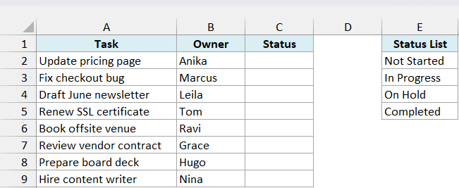
Below is the same task tracker with the Status List in E2:E5.

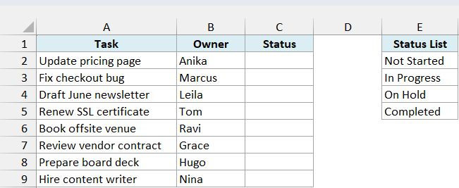
Here are the steps:

1. Select C2:C9, click the Data tab, and then click Data Validation.

2. In the Settings tab, select List in the Allow drop-down.

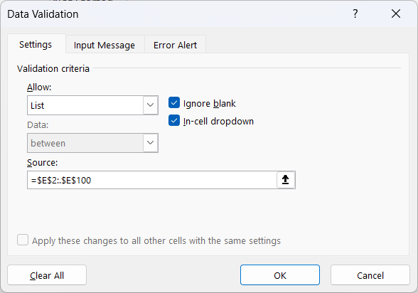
3. In the Source field, enter the following:

=$E$2:.$E$100

4. Click OK.

Note the dot right after the colon (:.). This is what tells Excel to drop the empty cells at the end of the range.

Now when you add a new status right below the last item, it shows up in the drop-down automatically (as long as it is within E100).

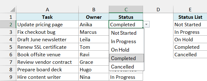
Unlike the OFFSET method below, this one still picks up every item even if there’s a blank cell somewhere in the middle of the list.

The TRIMRANGE function does the same thing, so =TRIMRANGE($E$2:$E$100) also works in the Source field. Both are available only in Microsoft 365.

Dynamic Drop Down List Using OFFSET (Older Excel Versions)

Apart from selecting cells and typing items, you can also use a formula in the Source field. Any formula that returns a list of values can be used to create a drop-down list.

In older versions of Excel, the classic way to make the drop-down update on its own is a formula that uses the OFFSET function with COUNTIF.

Below is the same task tracker with the Status List in E2:E5.

Here are the steps:

1. Select C2:C9, click the Data tab, and then click Data Validation.

2. In the Settings tab, select List in the Allow drop-down.

3. In the Source field, enter the following formula:

=OFFSET($E$2,0,0,COUNTIF($E$2:$E$100,"<>"))

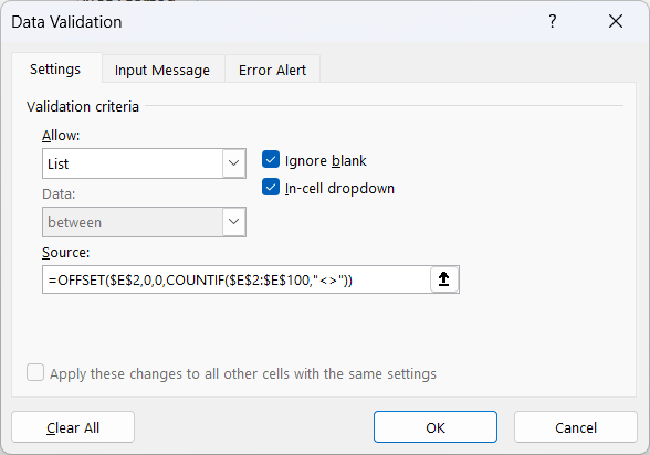
4. Click OK.

This creates a drop-down list that shows all four statuses, and it picks up any new status you add below E5.

How this formula works:

• The syntax of the OFFSET function is =OFFSET(reference, rows, cols, [height], [width]).
• The reference is E2, the starting point of the list. Rows and cols are 0, as we don’t want to move away from E2.
• The height is COUNTIF($E$2:$E$100,”<>”), which uses the COUNTIF function to count the non-blank cells in E2:E100. Right now, that’s 4.
• So the formula returns the four cells starting from E2 (E2:E5). When you add a fifth item, the count becomes 5, and the range grows to E2:E6.

If you had a fixed number of items, you could also use a plain number for the height, such as =OFFSET($E$2,0,0,4). But then the drop-down wouldn’t update when the list changes.

To see what the formula returns, enter it in any empty cell. In Microsoft 365, it spills the full list.

In older versions, select the formula in the formula bar and press F9 to see the array of items.

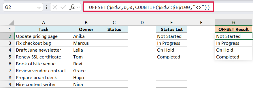
Important: For this to work, there must NOT be any blank cells in between the filled cells. A blank cell makes the count one short, and the last item drops out of the drop-down.

If you’re on Excel 2007 or later, the Excel Table method gives you the same result without a formula.

Use a Formula to Create a Sorted Drop Down List of Unique Items

Sometimes the items you want in the drop-down are in a column that has repeats. For example, below I have a project assignment log where each project appears more than once.

I want a drop-down in column B that shows each project only once, sorted A to Z.

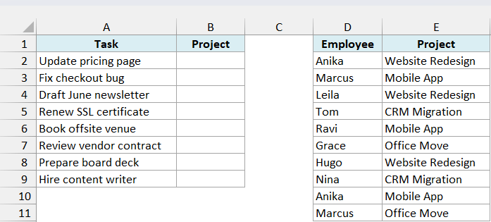
If you’re on Microsoft 365, the drop-down already removes the repeats for you. If you point it directly at E2:E11, each project shows up only once.

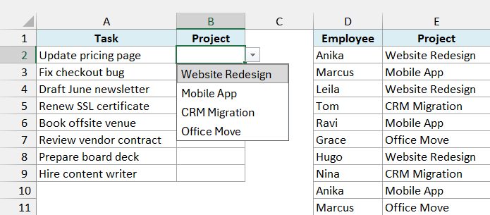
But there are two catches. The items stay in the order they appear in the column (they’re not sorted), and a blank cell in the range still shows up as an empty row.

Also, this is a fairly recent change in Microsoft 365. Older versions, such as Excel 2019, show every repeat in the drop-down.

So if you want a sorted list, or your file will also be opened in a version without this change, it’s better to build the list with a formula.

The UNIQUE function with SORT can give you this list. But you can’t put this formula directly in the Source field.

Important: If you type =SORT(UNIQUE(E2:E11)) in the Source field, Excel shows an error. The Source field doesn’t accept these functions directly.

The workaround is to put the formula in a cell first, and then point the drop-down to its result.

Here is the formula I’ve entered in cell G2:

=SORT(UNIQUE(E2:E11))

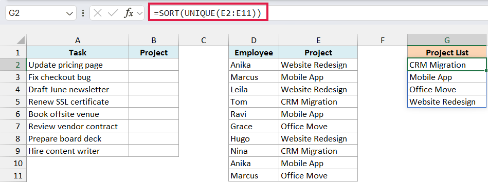
This returns the four projects in alphabetical order. The result spills down to G5 on its own, so you don’t need to copy the formula.

Now here are the steps to use this list in the drop-down:

1. Select B2:B9, click the Data tab, and then click Data Validation.

2. In the Settings tab, select List in the Allow drop-down.

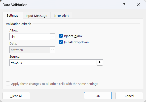
3. In the Source field, enter the following:

=$G$2#

4. Click OK.

The # after G2 is the spill range operator. It refers to the whole result of the formula in G2, however many rows that is.

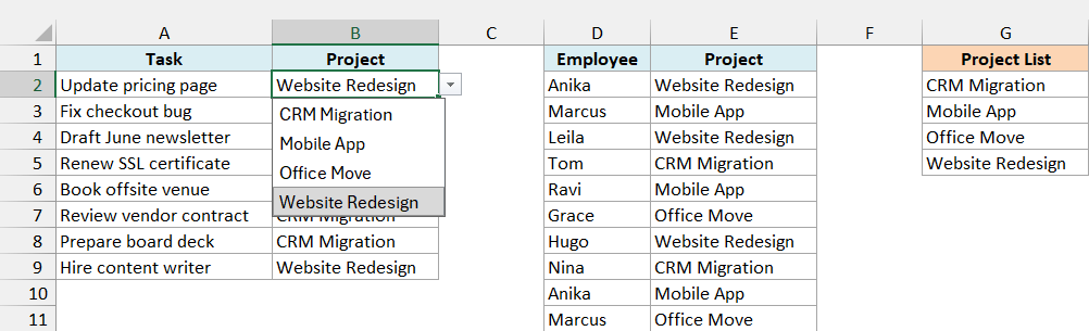
So if the formula returns five projects tomorrow, the drop-down shows five projects. This works in Excel 2021, Excel 2024, and Microsoft 365.

The formula above uses a fixed range (E2:E11). If your log keeps growing, point the formula at a Table column or use a trim reference (E2:.E100) so new entries are included.

You can use the same trick with any formula that returns a list, such as FILTER.

Copy a Drop Down List to Other Cells

You can copy and paste a cell that has a drop-down list, and the drop-down gets copied as well.

For example, if you have a drop-down list in C2 and you want it in C3:C9 as well, simply copy C2 and paste it in C3:C9.

Along with the drop-down, this also copies the value and formatting of C2.

If you only want to copy the drop-down, here are the steps:

1. Copy the cell that has the drop-down.

2. Select the cells where you want the drop-down.

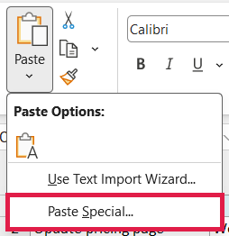
3. Go to Home, click the Paste drop-down, and click Paste Special (or press Ctrl + Alt + V).

4. In the Paste Special dialog box, select Validation.

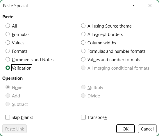
5. Click OK.

This copies only the drop-down, and not the value or formatting of the copied cell.

You need to be careful when copying the other way round, though.

Important: If you copy a cell without a drop-down and paste it over a cell that has one, the drop-down is gone. Excel doesn’t show any warning when this happens.

So it helps to know exactly which cells have a drop-down before you paste anything.

How to Find All Cells That Have a Drop Down List

In a large sheet, it’s hard to tell which cells have a drop-down list. The arrow only shows up when you select the cell.

Instead of checking each cell, there is a quick way to select all the cells that have a drop-down list (or any other data validation rule) in one go.

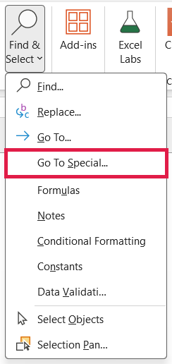
1. Go to Home, click Find & Select, and then click Go To Special.

2. In the Go To Special dialog box, select Data validation.

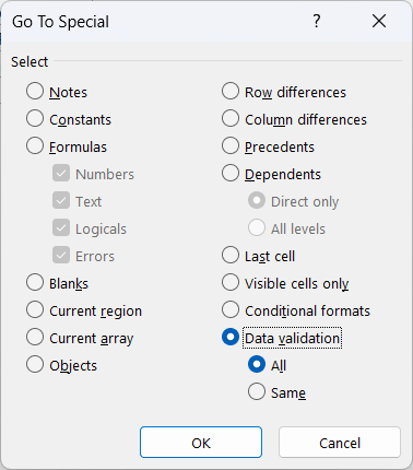
Data validation has two options below it: All and Same.

All selects every cell that has a data validation rule. Same selects only the cells that have the same rule as the active cell.

3. Click OK.

This instantly selects all the cells that have a data validation rule, and this includes drop-down lists.

Now you can give these cells a border or a background color, so they’re easy to spot and you don’t accidentally paste over them.

Here is another technique by Jon Acampora you can use to always keep the drop-down arrow visible. You can also see some ways to do this in this video by Mr. Excel.

Make the Second Drop Down Depend on the First

Sometimes, you want the items in a second drop-down to depend on what’s selected in the first one. These are called dependent or conditional drop-down lists.

Here is a video on how to create a dependent drop-down list in Excel.

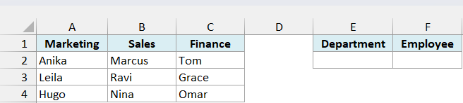
Below I have the employees of three departments in columns A to C. When I pick Sales in E2, I want the drop-down in F2 to show only the Sales team.

The classic way to do this uses named ranges and the INDIRECT function:

• Select A1:C4, go to Formulas, and click Create from Selection (or press Control + Shift + F3). Check only Top row. This creates three named ranges: Marketing, Sales, and Finance.
• The first drop-down in E2 uses =$A$1:$C$1 as the source, so it lists the three departments.
• The second drop-down in F2 uses =INDIRECT(E2) as the source.

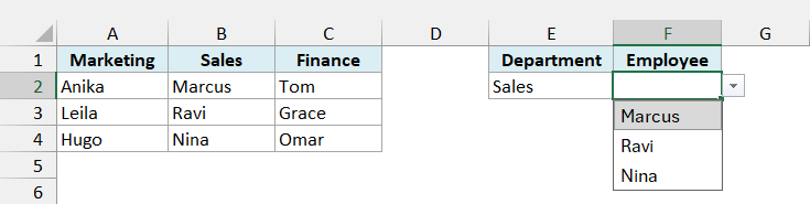
When you select Sales in E2, INDIRECT(E2) refers to the named range Sales, so the drop-down in F2 lists Marcus, Ravi, and Nina.

If a department name has more than one word (such as Human Resources), Excel names the range Human_Resources.

That’s because a named range can’t have spaces, so Excel swaps each space for an underscore.

In that case, use =INDIRECT(SUBSTITUTE(E2,” “,”_”)) instead, where the SUBSTITUTE function swaps the spaces for underscores.

Also note that if you change the first drop-down after making a selection in the second one, the second one doesn’t clear on its own.

It keeps the old name, which is now a wrong entry. Here is a great tutorial by Debra on clearing dependent drop-downs when the selection changes.

For the full step-by-step method, a newer way that doesn’t need INDIRECT, and multi-level drop-downs, see how to create a dependent drop-down list in Excel.

So these are the ways you can create a drop-down list in Excel, from a simple list of cells to one that updates on its own as your list grows.

I hope you found this Excel tutorial useful.

Other Excel tutorials you may also like:

• Extract Data from Drop Down List Selection in Excel
• Select Multiple Items from a Drop Down List in Excel
• Creating a Dynamic Excel Filter Search Box
• Display Main and Subcategory in Drop Down List in Excel
• How to Insert Checkbox in Excel
• Using a Radio Button (Option Button) in Excel
• How to Remove Drop-Down List in Excel?
• Create Data Validation List from Excel Table as Source
• Creating Multiple Drop-down Lists in Excel without Repetition
• Excel Data Entry Tips