

One of the Excel queries I often get is – “How to highlight the Active Row and Column in a data range?”
And I got one last week too.

So I decided to create a tutorial and a video on it. It will save me some time and help the readers too.
Below is a video where I show how to highlight the active row and column in Excel.
In case you prefer written instructions, below is a tutorial with exact steps on how to do it.
Let me first show you what we are trying to achieve.
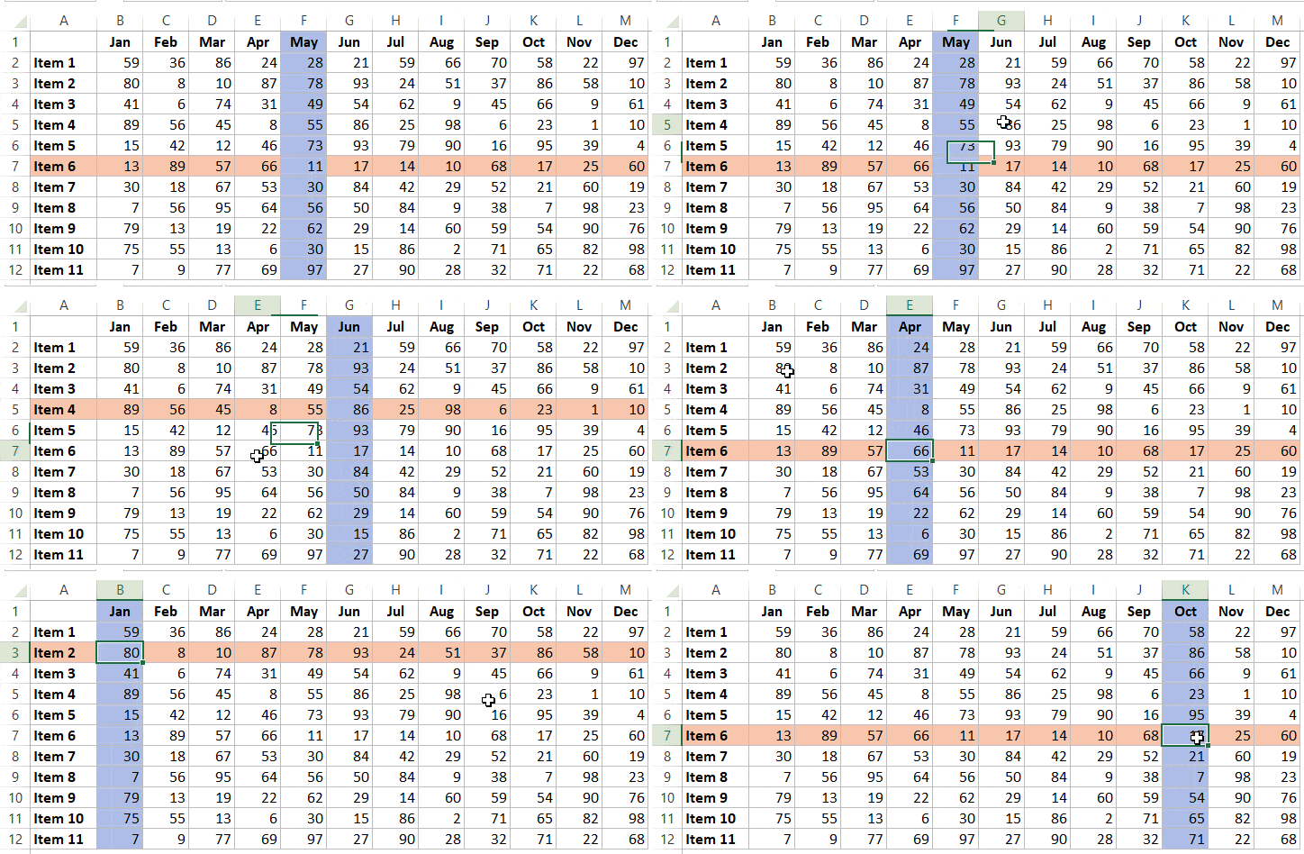
In the above example, as soon as you select a cell, you can see that the row and column also get highlighted. This can be helpful when you’re working with a large dataset and can also be used in Excel Dashboards.
Now let’s see how to create this functionality in Excel.
Highlight the Active Row and Column in Excel
Here are the steps to highlight the active row and column on selection:
- Select the data set in which you to highlight the active row/column.
- Go to the Home tab.
- Click on Conditional Formatting and then click on New Rule.
- In the New Formatting Rule dialog box, select “Use a formula to determine which cells to format”.
- In the Rule Description field, enter the formula: =OR(CELL(“col”)=COLUMN(),CELL(“row”)=ROW())
- Click on the Format button and specify the formatting (the color in which you want the row/column highlighted).
- Click OK.
The above steps have taken care of highlighting the active row and active column (with the same color) whenever there is a selection change event.
However, to make this work, you need to place a simple VBA code in the backend.
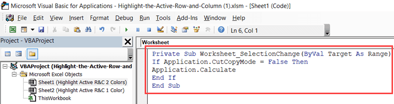
Here is the VBA code that you can copy and paste (exact steps also listed below):
'Code developed by Sumit Bansal from https://trumpexcel.com
Private Sub Worksheet_SelectionChange(ByVal Target As Range)
If Application.CutCopyMode = False Then
Application.Calculate
End If
End Sub
The above VBA code is run whenever there is a selection change in the worksheet. It forces the workbook to recalculate, which then forces the conditional formatting to highlight the active row and the active column.
Normally (without any VBA code), a worksheet refreshes only when there is a change in it (such as data entry or edit).
Also, an IF statement is used in the code to check if the user is trying to copy-paste any data in the sheet.
During copy-paste, the application is not refreshed, and it is allowed.
Here are the steps to copy this VBA code in the backend:
- Go to the Developer tab (can’t find the developer tab? – read this).

- Click on Visual Basic.

- In the VB Editor, on the left, you will see the project explorer that lists all the open workbooks and the worksheets in it. If you can’t see it, use the keyboard shortcut Control + R.

- With your workbook, double-click on the sheet name in which you have the data. In this example, the data is in Sheet 1 and Sheet 2.
- In the code window, copy and paste the above VBA code. You’ll have to copy and paste the code for both sheets if you want this functionality in both sheets.
- Close the VB Editor.
Since the workbook has VBA code in it, save it with a .XLSM extension.
Note that in the steps listed above, the active row and column would get highlighted with the same color. If you want to highlight the active row and column in different colors, use the below formulas:
- =COLUMN()=CELL(“col”)
- =CELL(“row”)=ROW()
In the download file provided with this tutorial, I have created two tabs, one each for single color and dual color highlighting.
Since these are two different formulas, you can specify two different colors.
Useful Notes:
- This method would not impact any formatting/highlighting you have done manually to the cells.
- Conditional formatting is volatile. If you use it on very large datasets, it may lead to a slow workbook.
- The VBA code used above would refresh the workbook every time there is a change in selection.
- CELL Function is available in Excel 2007 and above version for Windows and Excel 2011 and above for Mac. In case you’re using an older version, use this technique by Chandoo.
Want to Level-up your Excel Skills? Consider joining one of my Excel courses:
You May Also Like the Following Excel Tutorials:

Very Good and thank you.
One small issue was that i found copying the formula in it’s BOLD format caused it not to work. I had to re-write it in normal text and it worked fine.
Very good book. Useful for excel beginners
Searching this long grt tutorial and suffer one error also but with someone comment i change according n its work
here he typed:
=OR(CELL(“col”)=COLUMN(),CELL(“row”)=ROW())
everything needs to be caps so:
=OR(CELL(“COL”)=COLUMN(),CELL(“ROW”)=ROW())
thanks for your efforts, but i think Microsoft should add this as a basic excel services , no need to do this long steps
How to enable that please tell me.
Forgot one important thing. I am using Windows 10, 64 bit, Excel office 365.
This is what I wanted. But, it only works on 1 worksheet in my workbook of 10 sheets. I have copied the VBA code on 2 or 3 sheets to see if that works, but still only works on 1 sheet. I would like to be able to not only work on all sheets, but also any other workbook file I need to use it in. Can you help me? Also, is it possible to make this an Excel Add-in, so it would work in any file I open?