
If you work with phone numbers data in Excel, it would be useful to know how to properly format them.
For example, if you’re working with phone numbers in the US, instead of just showing a 10-digit screen, you can format it to show in the following format:
(123) 456-7890
If you are working with phone number data of any other country, you can easily customize the phone.
In this tutorial, I’ll show you several ways to format phone numbers in Excel. We’ll start with simple custom formatting when your data is clean data and move to advanced formulas for messy phone number datasets with extensions and random characters (such as space or hyphen or dot).
So let’s get to it!
Click here to download the example file
Example 1: Using Custom Number Formatting (For Clean Numeric Data)
If you have phone numbers as proper numeric data in your Excel file, it’s pretty easy to format it using custom number formatting.
Let me explain with an example.
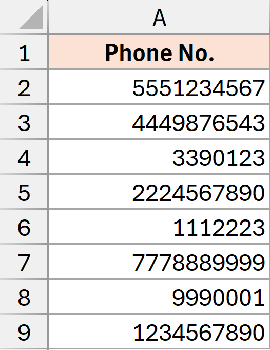
Below, I have a dataset where I have the phone numbers in Column A, and these are stored as numbers in Excel (which is evident by the fact that these are aligned to the right by default).
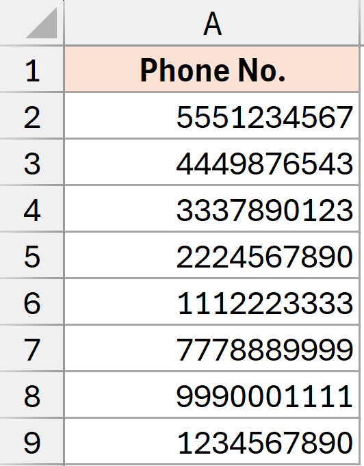
Since this is a numeric data set, I can apply custom number formatting on this data to make these numbers appear in a desired format.
Here are the steps to change the custom number formatting to make these numbers show up as proper phone number formats.
- Select the range that contains the phone numbers
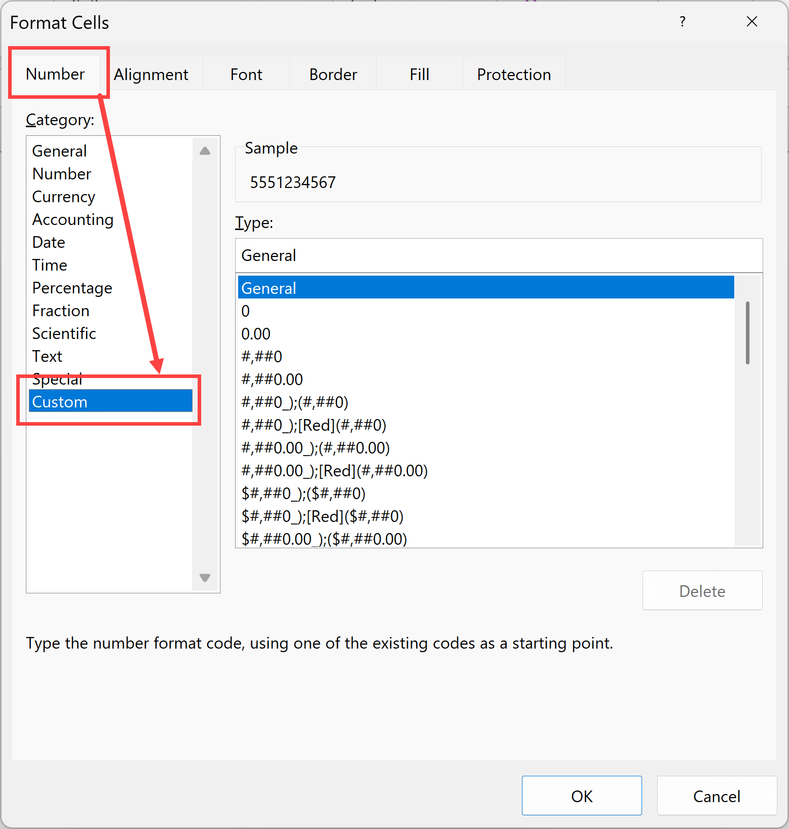
- Press Ctrl + 1 to open the Format Cells dialog box
- In the Format Cells dialog box, select the Number tab, then select Custom option in the category list
- Enter this format code
(###) ###-####
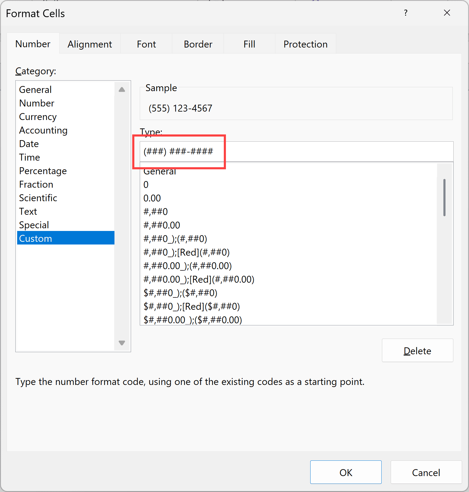
- Click OK
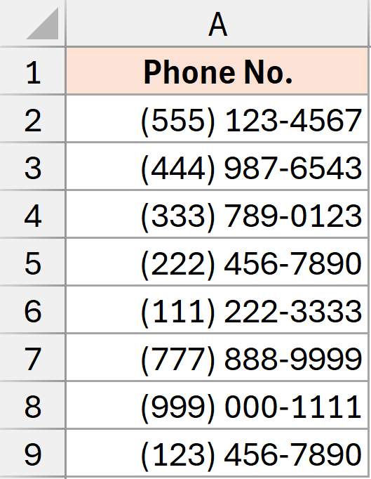
The above steps would format the numbers so that it appears as shown below.
Explanation for the custom formatting code:
- ( and ) – These will appear as literal parentheses
- Each # represents a digit from your number
- Space and – appear as literal characters
The result will show the number 5551234567 as (555) 123-4567
When you apply custom number formatting to a cell, it only changes how the value in the cell appears to you. It doesn’t change the actual value in that cell. So while you may see (555) 123-4567 as the result, the actual value in the backend would be 5551234567
Note: This method only works with numerical data. If your phone numbers are stored as text (indicated by left alignment in the cell), you’ll need to convert them to numbers first or use the formula methods covered in Example 3.
Click here to download the example file
Various Custom Number formatting Examples for Phone Numbers
Here are some other custom formatting ideas you can use when formatting your phone number:
To get the country code along with the phone number:
+1 (###) ###-####
or
001 (###) ###-####
To have dot as a separator in phone number:
###\.###\.####
Also read: Convert Text to Numbers in Excel
Example 2: Using Conditional Custom Number Formatting (7 & 10 Digit Numbers)
Another common example of phone number data in the U.S. is when you have a mix of 7-digit and 10-digit numbers.
This is usually the case when a 3-digit state code is included in some of the numbers but not in the others.
Below I have a dataset in column A where I have a mix of 7-digit and 10-digit numbers and I want to format it like phone numbers.
Here are other steps to format these as phone numbers:
- Select the range that contains the phone numbers
- Press Ctrl + 1 to open the Format Cells dialog box
- In the Format Cells dialog box, select the Number tab, then select Custom option in the category list
- Enter the format code below:
[>9999999](###) ###-####;###-####
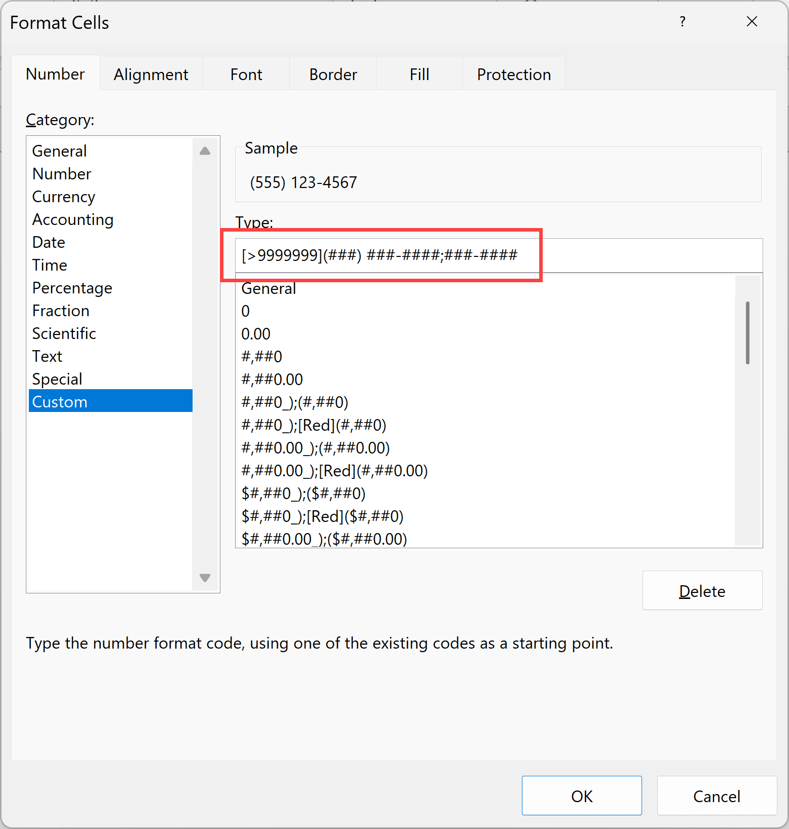
- Click OK
The above steps would format the numbers so that it appears as shown below.
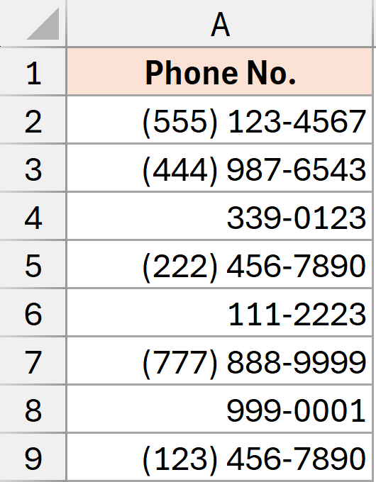
The above is a conditional custom formatting code that has two conditions; one before the semicolon and one after the semicolon.
Each value is checked for the condition [>9999999] and if the number is more than 7 digits, ### ###-#### format is applied to it.
And all the other cases, ###-#### format is applied to the cells.
Click here to download the example file
Example 3: Using TEXT Function (For Phone Numbers in Text Format)
If some or all of the numbers in cells are text values, then you cannot use the custom number formatting method covered earlier.
In that case, you can use the TEXT function method I cover here.
Below I have a dataset where some of the phone numbers are in the text format (which is why there is a line to the left in the cell).
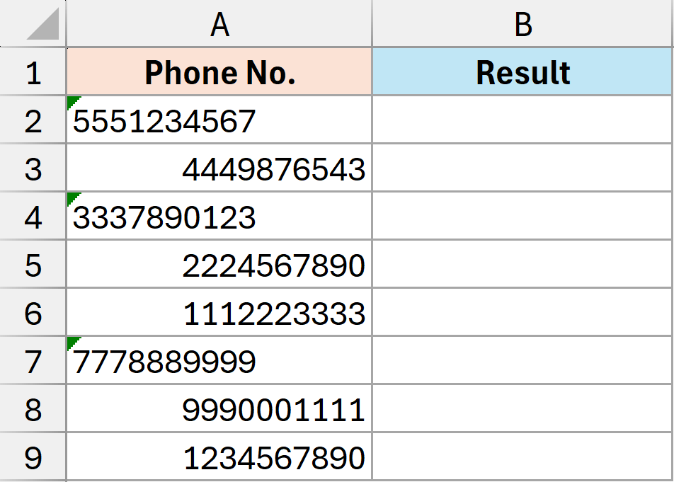
To format all of these numbers as proper phone numbers, we can use the below formula.
=TEXT(A2:A9,"(###) ###-####")
Enter this formula and cell B2, it will spill the results in the entire column to give you the numbers in the specified phone number format.
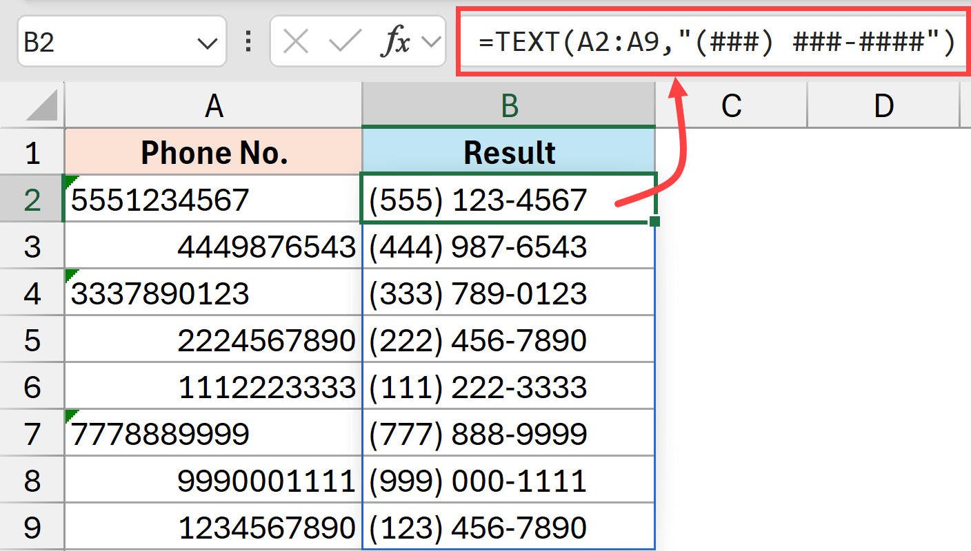
The TEXT function works by taking the value in a cell as the first argument and then applying the format that is specified as the second argument. Note that the format in the second argument should always be within double quotes.
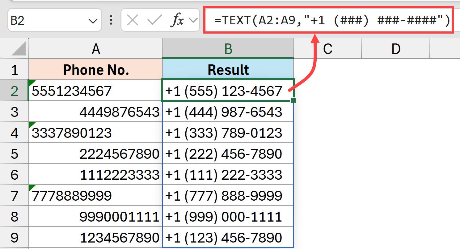
If you want to show the country code along with the phone number, then you can use the below formula.
=TEXT(A2:A9,"+1 (###) ###-####")
Example 4: Formatting Phone Numbers of Varying Length
Sometimes you may get phone numbers that are of varying length and also have spaces between the digits (something as shown below).
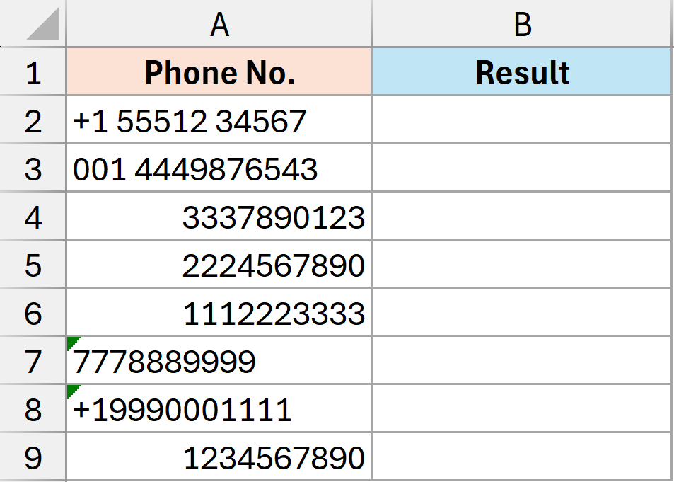
To format these numbers as proper phone numbers, we first need to get rid of any extra spaces in the cells and then extract the last 10 digits.
Here’s a formula that’ll do this.
=TEXT(RIGHT(SUBSTITUTE(A2:A9," ",""),10),"(###) ###-####")
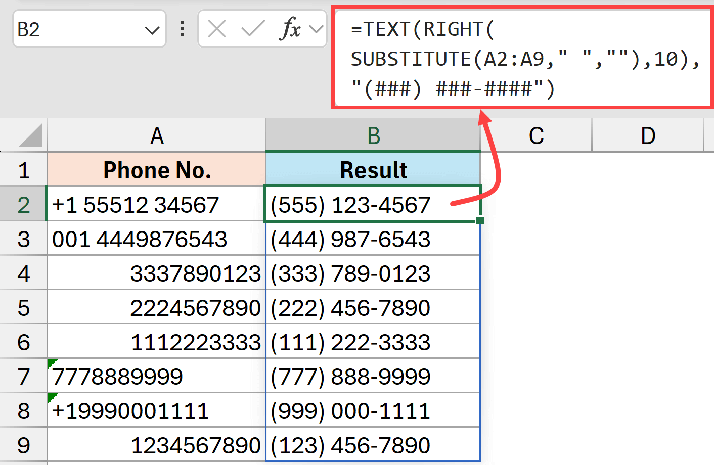
In the above formula, I first use the SUBSTITUTE function to get rid of all the spaces in the cell.
Once that is done, I have used the RIGHT function to extract the last 10 digits from each cell.
And when I have the last 10 digits, I can use the Text function to format it as a proper phone number.
With this formula, it removes the country codes and any other additional characters that are there before the phone number, giving me only a 10-digit phone number.
If you now want to add a country code to this result, you can do that by modifying the custom number format within the TEXT function.
For example, if you want to add +1 as the country code and all these numbers, you can use the below formula:
=TEXT(RIGHT(SUBSTITUTE(A2:A9," ",""),10),"+1 (###) ###-####")
Click here to download the example file
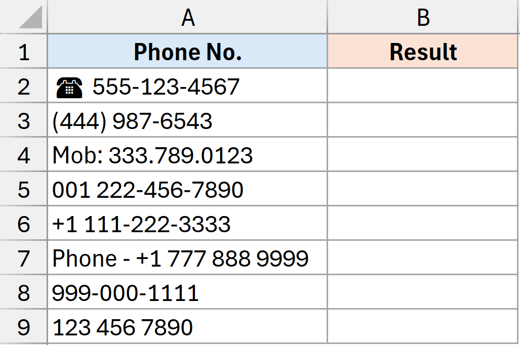
Example 5: Formatting Messy Phone Number Data (with Spaces, Dots, Hyphens, Text)
In some cases, you may end up with messy phone number data as (shown below) that has additional characters such as spaces, dots, hyphens, or even words along with the phone number.
Since there is no consistency in the data, it would be it would be very difficult to extract only the digits from this data using regular text functions in Excel.
Thankfully, now there are new REGEX functions in Excel with Microsoft 365 that can do this easily.
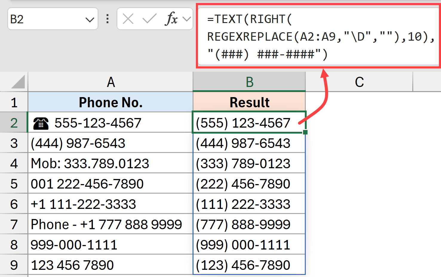
Below is the formula that will extract the digits from the cell and then format it as a phone number.
=TEXT(RIGHT(REGEXREPLACE(A2:A9,"\D",""),10),"(###) ###-####")
Let me explain the formula:
- REGEXREPLACE(A2:A9,”\D”,””) – This part of the formula replaces anything which is not a digit by a blank string (\D is the meta character that represents any character that is not a digit).
- RIGHT(REGEXREPLACE(A2:A9,”\D”,””),10) – Once I have only the digits from each cell, RIGHT function extracts the last 10 digits from each cell.
- TEXT(RIGHT(REGEXREPLACE(A2:A9,”\D”,””),10),”(###) ###-####”) – The text function is now used over the result returned by the RIGHT function to apply the format to the 10 digits in each cell.
Note: Excel has three new REGEX functions (REGEXEXTRACT, REGEXREPLACE, and REGEXTEST, and these are available in Excel in Microsoft 365 and Excel on the web. These are not available in the older versions of Excel.
Click here to download the example file
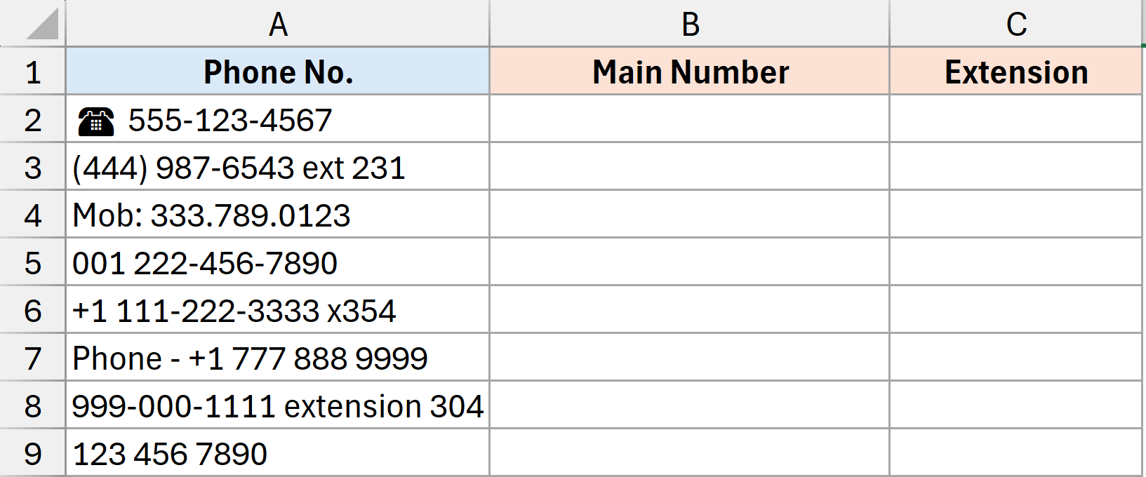
Example 6: Formatting Messy Phone Number Data (with Extension)
In this example, I have messy phone number data along with the extensions as shown below.
I can’t use the REGEXREPLACE function used in previous example because it won’t be able to differentiate between the main phone number and the digits in the extension.
In this case, I would have to extract the extension and the main phone number separately by using the TEXTBEFORE and TEXTAFTER functions.
Here is the formula to extract the extension:
=IFERROR(TRIM(TEXTAFTER(A2:A9,{"ext";"x";"extension"})),"")
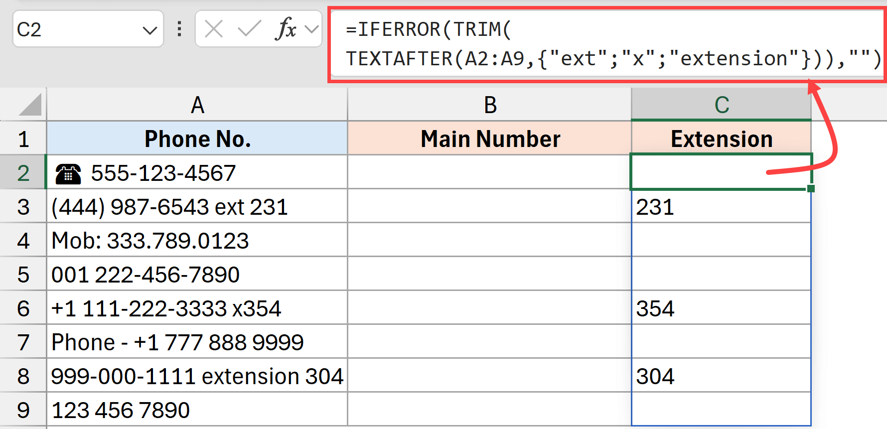
The above formula uses “text after” with multiple delimiters in curly brackets to extract anything that comes after ext or x or extension. TRIM function is used to ensure there are no leading or trailing spaces.
And then IFERROR is used to remove the error in case there is no extension in the cell.
And here is the formula that will extract the main phone number before the extension and format it as a proper phone number.
=TEXT(RIGHT(REGEXREPLACE(IFERROR(TRIM(TEXTBEFORE(A2:A9,{"ext";"x";"extension"})),A2:A9),"\D",""),10),"(###) ###-####")
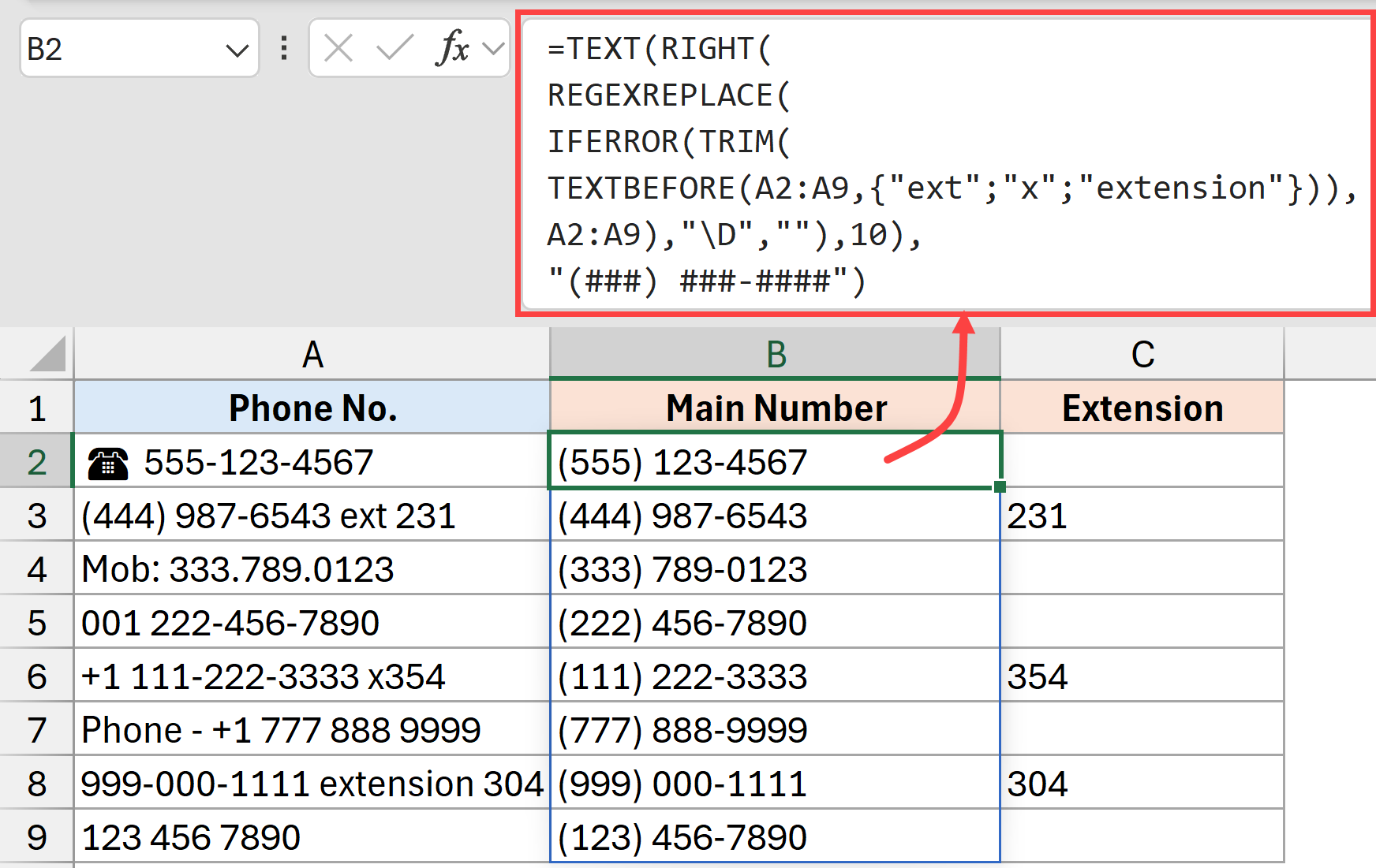
The above formula uses the same logic along with the TEXTBEFORE function to extract anything that is before ext or x or extension.
Once we have everything before the extension number, we can use the REGEXREPLACE function to extract only the digits, then use the RIGHT function to extract the last 10 digits and then use the TEXT function to apply the phone number format.
In this article, I’ll show you various examples on how to format phone numbers in Excel. If you have basic numeric data, you can quickly apply the custom number formatting on the data. If you have the data as text values, then you can use the TEXT function to do it.
And in case you have messy phone number data that may have spaces or characters such as. or – or [ ] or even words, then you can use REGEX functions to first extract the digits and then format these as needed.
I hope you found this article helpful. In case you have any questions or suggestions for me, please let me know in the comment section.
Other Excel articles you may also like:


