XMATCH Function in Excel

When you need to know the position of a specific item in a list, you can use the XMATCH function in Excel. It returns the position as a number, which you can then use with functions like INDEX to look up a value.

In this article, I’ll show you how to use XMATCH in Excel with eight examples, including last matches, partial matches, and custom sorting.

Excel XMATCH Function Syntax

Here is the syntax of the XMATCH function:

=XMATCH(lookup_value, lookup_array, [match_mode], [search_mode])

• lookup_value is the value you want to find. This can be text, a number, a cell reference, or a range of values to look up together.
• lookup_array is the one-row or one-column array or range you want to search. XMATCH counts positions from the start of this array.
• match_mode is optional. Use 0 for an exact match (the default). With no exact match, -1 finds the next smaller item, while 1 finds the next larger item. Use 2 for wildcard matching with *, ?, and ~.
• search_mode is optional. Use 1 to search first to last (the default), or -1 to search last to first. Modes 2 and -2 do a binary search, which only works correctly on sorted data.

If you leave both optional arguments out, XMATCH looks for an exact match and searches from first to last.

The one thing to keep in mind: XMATCH returns a position within the lookup array. It doesn’t return the value there or the worksheet row number.

When to Use the XMATCH Function

Use the XMATCH function when you need to:

• Find where an item sits in a row or column when the position itself is the answer.
• Get positions for several items at once with one spilling formula.
• Find the first or last occurrence of a repeated value.
• Find the next larger or smaller value without sorting the lookup data.
• Locate partial-text matches or the first row that meets multiple conditions.
• Feed positions into INDEX, FILTER, or SORTBY for a lookup, missing-item list, or custom sort.

Let me show you a few practical examples of how this works.

Example 1: Find Positions for Several Performers

Let’s start by finding several positions with one formula.

Below is a school concert running order with 12 performers, and I want the slots for Bao, Siobhan, Femi, and Anouk in column E.

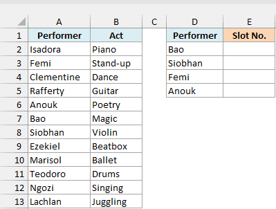
Here is the formula:

=XMATCH(D2:D5,A2:A13)

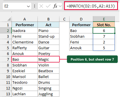
Because you gave XMATCH the whole range D2:D5, it looks up all four names. The results spill into E2:E5: 6, 7, 2, and 5.

Bao is sixth in A2:A13, so XMATCH returns 6. Bao’s worksheet row is 7, but that’s not what the formula counts.

No third argument is needed because XMATCH matches exactly by default. The older MATCH function needs 0 for an exact match.

If anything is in E3:E5, Excel returns #SPILL! because it has no room for the other three results. Clear those cells before entering the formula.

XMATCH works in Microsoft 365, Excel 2024, and Excel 2021 on Windows and Mac, plus Excel for the web. Excel 2019 and earlier return #NAME?.

If you are using Excel 2019 or earlier, use MATCH instead. Enter the below formula in cell E2 and then copy it down to E5:

=MATCH(D2,$A$2:$A$13,0)

Example 2: Find When Savings Goals Are Reached

Now let’s find a position when the exact number isn’t in the list.

Below is a 12-week savings tracker with running totals, and I want the first week each savings goal is reached in column F.

The goals are $500, $1,000, and $1,250.

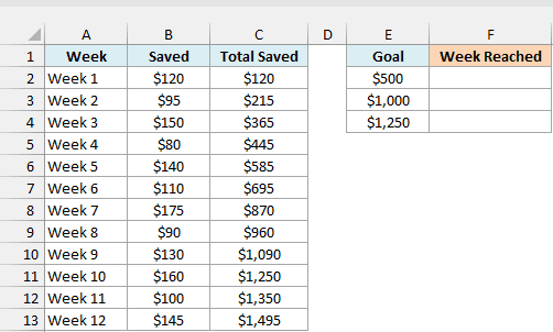
Here is the formula:

=XMATCH(E2:E4,C2:C13,1)

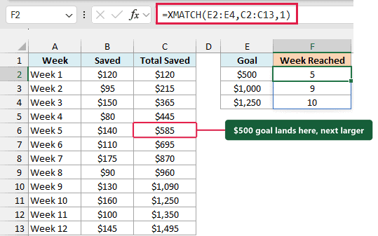
The results spill into F2:F4: 5, 9, and 10. The 1 in the third argument means exact match or next larger item.

There’s no $500 total, so XMATCH finds $585 in Week 5.

For $1,000, it finds $1,090 in Week 9. The $1,250 goal matches Week 10 exactly.

Using match_mode -1 would find an exact match or the next smaller item. For $500, that would be $445 in Week 4.

Here, the position also happens to be the week number because C2 is Week 1. XMATCH is still returning a position, rather than the text label.

To return “Week 5” itself, use XLOOKUP with the Week column as the return array.

One nice thing here is that XMATCH doesn’t need the totals to be sorted for this to work. That’s not the case with the older MATCH function.

Important: MATCH’s mode 1 means exact or next smaller and needs ascending data. XMATCH’s mode 1 means exact or next larger, so changing functions can change the answer.

Example 3: Find the Last Match (search_mode -1)

Now let’s flip the search direction to find the last match.

Below is a book club attendance sheet for eight members and eight meetings, and I want each member’s last meeting number in column J.

A “Yes” means the member attended; other attendance cells are blank.

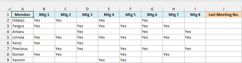
Here is the formula:

=XMATCH("Yes",B2:I2,0,-1)

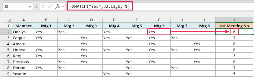
Enter it in J2 and copy it down to J9 to get the last meeting for each member.

The 0 keeps an exact match, and the fourth argument, -1, searches from the end. For Odalys, it finds the last “Yes” at meeting 6.

XMATCH works across a row just as well as down a column. Here, the position in B2:I2 is the meeting number because B2 is meeting 1.

We copy this one down because each member has a separate row to search. You could make it spill with the BYROW and LAMBDA functions, but the formula gets a lot harder to read.

This is also useful when you need to find the last occurrence of an item in a list, which MATCH can’t do because it has no reverse search.

Example 4: Find Partial Matches with Wildcards

Let’s look for a word inside a longer book title.

Below is a top 10 bestseller list, and I want the rank of the first title containing each keyword, or a message if none matches, in column E.

The keywords are Garden, Moon, kitchen, and Ocean.

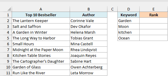
Here is the formula:

=IFNA(XMATCH("*"&D2:D5&"*",A2:A11,2),"Not in top 10")

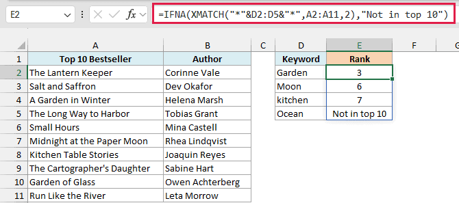
The results spill into E2:E5: 3, 6, 7, and “Not in top 10”.

Here is how this formula works:

• "*"&D2:D5&"*" joins an asterisk to each side of every keyword. Garden becomes *Garden*, which matches a title containing Garden anywhere.
• The third argument, 2, switches on wildcard matching. Without it, XMATCH treats the asterisks as literal characters.
• XMATCH returns the first matching position for each keyword. Garden appears at ranks 3 and 9, so the result is 3.
• Ocean doesn’t appear in any title, so XMATCH returns #N/A. IFNA replaces that error with “Not in top 10”. The other results pass through unchanged.

Also note that XMATCH isn’t case sensitive, which is why the lowercase kitchen still finds Kitchen Table Stories at rank 7.

If you need the letter case to match too, use XMATCH with the EXACT function, like =XMATCH(TRUE,EXACT(lookup_value,lookup_array)).

EXACT returns TRUE only where both the text and its case match, and XMATCH finds the first TRUE.

If your pattern needs to match just one character, use ?, one of Excel’s wildcard characters.

If you want an actual asterisk or question mark in the text, use ~* or ~? so Excel treats it as a literal character.

Pro Tip: In Microsoft 365 (not Excel 2021 or 2024), match_mode 3 lets you match with regular expressions. See the REGEX functions guide for pattern examples.

Example 5: XMATCH with Multiple Criteria

You can also find the first position where two conditions are true together.

Below is a fitness log for 12 days, and I want the first day that meets both the step and sleep goals in F3.

The step goal in F1 is 10,000, and the sleep goal in F2 is 8 hours.

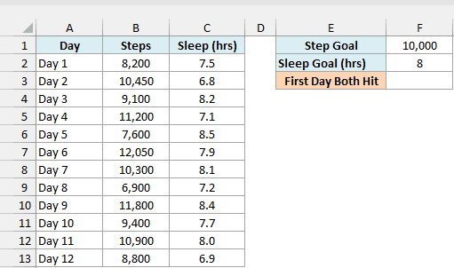
Here is the formula:

=XMATCH(1,(B2:B13>=F1)*(C2:C13>=F2))

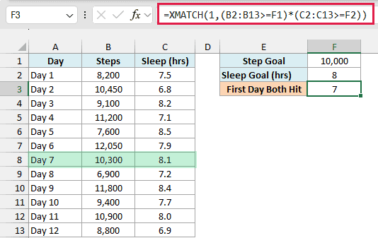
This returns 7. Day 7 is the first day with at least 10,000 steps and 8 hours of sleep: 10,300 steps and 8.1 hours.

Here is how this formula works:

• B2:B13>=F1 checks the step goal and returns TRUE or FALSE for each day.
• C2:C13>=F2 does the same for the sleep goal.
• Multiplying the two sets of results turns TRUE/FALSE into 1/0. A row gives 1 only when both conditions are TRUE; every other row gives 0.
• XMATCH looks for the first 1 in that array and returns its position, which is 7.

Earlier days meet only one goal. Days 2, 4, and 6 meet the step goal, while Days 3 and 5 meet the sleep goal.

Change F1 or F2, and the answer updates.

If a day should count when either goal is met, add the two conditions instead of multiplying them. A day then scores 1 or 2, so check for a score of at least 1:

=XMATCH(TRUE,((B2:B13>=F1)+(C2:C13>=F2))>=1)

Example 6: Find Who Hasn’t Checked In

Now let’s use missing matches to return a list of people.

Below are team workshop lists with 12 RSVPs and eight check-ins, and I want the names and teams of people still to check in, in columns F and G.

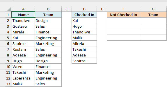
Here is the formula:

=FILTER(A2:B13,ISNA(XMATCH(A2:A13,D2:D9)),"Everyone checked in")

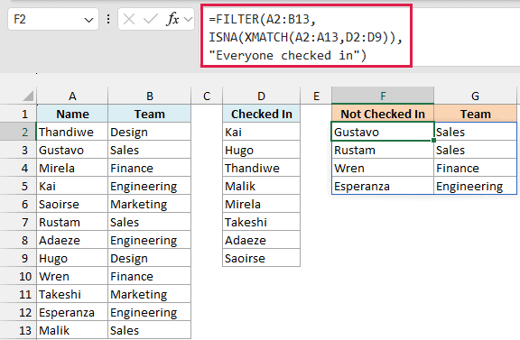
The result spills into F2:G5, listing the four people who haven’t checked in, along with their teams.

Here is how this formula works:

• XMATCH(A2:A13,D2:D9) looks up all 12 RSVP names in the checked-in list at once. It returns a position for a match and #N/A for a name it can’t find.
• ISNA turns each #N/A into TRUE. Names that were found return FALSE.
• FILTER keeps the rows from A2:B13 where ISNA returns TRUE, bringing back both the name and the team.
• The third FILTER argument, "Everyone checked in", supplies a message when nobody is missing.

The FILTER function returns the rows you need, while XMATCH and ISNA decide which people belong in that list.

Example 7: Two-Way Lookup with INDEX and XMATCH

Let’s use two positions to look up a price where a row and column meet.

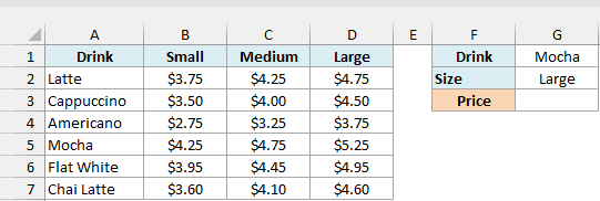
Below is a coffee price list for six drinks, and I want to look up the drink in G1 and size in G2, with the price in G3.

G1 holds Mocha and G2 holds Large, chosen from the Small, Medium, and Large sizes.

Here is the formula:

=INDEX(B2:D7,XMATCH(G1,A2:A7),XMATCH(G2,B1:D1))

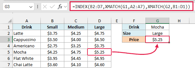
This returns $5.25, the price of a Large Mocha.

Here is how this formula works:

• XMATCH(G1,A2:A7) finds Mocha in the fourth position and returns 4, the row position within the price block.
• XMATCH(G2,B1:D1) finds Large in the third position and returns 3, the column position within that block.
• The INDEX function takes those two positions and returns the price where row 4 and column 3 intersect in B2:D7.

Change the drink in G1 or the size in G2, and the price updates. You don’t need to count the row or column yourself.

This follows the same idea as the classic INDEX and MATCH combination, with XMATCH supplying the positions.

You can also get the same price with two XLOOKUP functions, one inside the other:

=XLOOKUP(G2,B1:D1,XLOOKUP(G1,A2:A7,B2:D7))

The inner XLOOKUP returns Mocha’s three prices. The outer one picks the Large price from that row.

Example 8: Sort by a Custom Day Order

For the last example, let’s sort a schedule in weekday order.

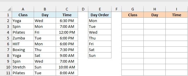
Below is a gym schedule with ten classes, and I want to sort it Monday to Sunday, then by time within each day, starting in column G.

The custom day order lists Mon through Sun.

Here is the formula:

=SORTBY(A2:C11,XMATCH(B2:B11,E2:E8),1,C2:C11,1)

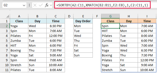
The sorted schedule spills into G2:I11, with Monday’s two classes at the top and Sunday’s Stretch at the bottom.

Here is how this formula works:

• XMATCH(B2:B11,E2:E8) turns each class’s day into its position in the custom list. Mon becomes 1, Tue becomes 2, and so on through Sun at 7.
• SORTBY sorts A2:C11 by those ranks. The first 1 means ascending order, so Monday’s classes appear first.
• The second sort pair, C2:C11,1, sorts by time in ascending order within each day.

An A to Z sort would put Fri first. XMATCH lets you supply the weekday order instead of relying on alphabetical order.

Change the order in E2:E8, and the table re-sorts to match.

To show the results as times, format the output Time column in I2:I11 with a time format, such as h:mm AM/PM.

Unlike SORT, which takes a column number to sort by, SORTBY can use the day ranks calculated inside this formula.

Use XMATCH when the position is the answer, or when another function needs that position. Start with an exact lookup, then change the match or search mode as needed.

List of All Excel Functions

Other Excel Articles You May Also Like:

• VLOOKUP vs XLOOKUP Function – What’s the Difference?
• Find the Closest Match in Excel
• How to Compare Two Columns in Excel
• How to use VSTACK in Excel
• Excel CHOOSE function
• LOOKUP Function in Excel
• VLOOKUP Function in Excel (10 Examples)
• SEARCH Function in Excel (7 Examples)