

If you want to combine text from several cells with a separator between each item, the TEXTJOIN function in Excel does that for you.
You pick the separator once, and it can skip empty cells as it goes.
TEXTJOIN returns one string without spilling, and it also works with dynamic array functions such as FILTER.
In this article, I’ll show you how to use TEXTJOIN in Excel with seven practical examples, starting with a simple list.
Follow along with the example file
TEXTJOIN Function Examples.xlsx
Excel TEXTJOIN Function Syntax
Here is the syntax of the TEXTJOIN function:
=TEXTJOIN(delimiter, ignore_empty, text1, [text2], ...)
- delimiter – Required. The separator between items, such as a comma, space, or hyphen. Use
""for no separator, a cell reference, or a number, which Excel treats as text. - ignore_empty – Required. TRUE skips empty cells so you don’t get repeated delimiters. FALSE keeps every position, even the blank ones.
- text1 – Required. The first item, cell, range, or array to join.
- [text2], … – Optional extra items or ranges. You can supply up to 252 text arguments in total, including text1.
The delimiter is inserted between items, never after the last one. So ", " adds a comma and a space between entries without leaving a comma at the end.
If you need different separators between items, you can supply the delimiters as a range or array. TEXTJOIN uses them in order, then starts again with the first.
For example, =TEXTJOIN({"-","/"},TRUE,"a","b","c","d") returns a-b/c-d, because the separators follow the order hyphen, slash, hyphen.
The ignore_empty switch decides what happens to blank cells. With TRUE, a blank cell is skipped entirely and no extra delimiter is added.
With FALSE, the blank still gets its slot, so delimiters appear back to back with nothing between them. Example 2 shows both results.
For text1 and the arguments after it, you can pass a single cell, a whole range, or several ranges. A range like A2:A11 counts as one argument, regardless of its size.
When to Use the TEXTJOIN Function
Use TEXTJOIN when you need to:
- Turn a column into a list separated by commas, spaces, or another delimiter.
- Build codes or labels from parts that may be missing.
- Stack items on separate lines inside one cell.
- Join dates and amounts into a readable summary.
- List every value that matches a condition, or each unique value, in one cell.
Let me show you a few practical examples of how this works.
Example 1: Turn a Column into a Comma-Separated List
Let’s start with a shopping list you can send in a text message.
Below is a grocery list with ten items, and I want to join them into one comma-separated line in C2.
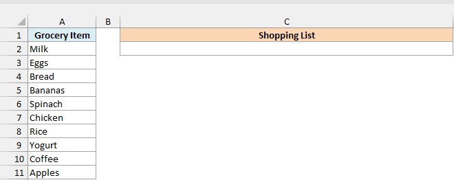
Here is the formula:
=TEXTJOIN(", ",TRUE,A2:A11)
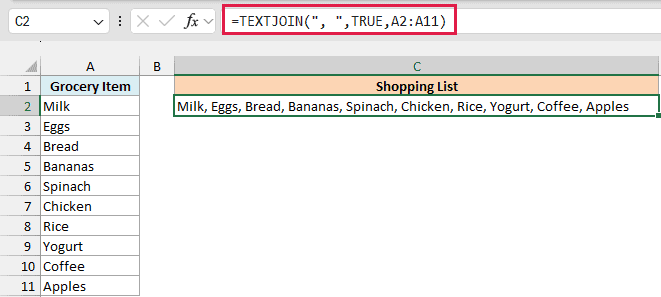
This returns Milk, Eggs, Bread, Bananas, Spinach, Chicken, Rice, Yogurt, Coffee, Apples.
In the above formula, ", " is the delimiter. It adds a comma and a space between the items, with nothing after Apples.
The whole range A2:A11 is one text argument, so you don’t have to list every cell separately. Add an item inside the referenced range and the list updates.
TEXTJOIN works in Excel for Microsoft 365, Excel 2024, 2021, 2019, and Excel for the web. It’s also available in Excel for Mac 2019 and later.
Excel 2016 and earlier don’t have TEXTJOIN, so those versions show #NAME?.
The result can’t exceed a cell’s 32,767-character limit. If it does, TEXTJOIN returns #VALUE!.
An error inside the joined range, such as #N/A, comes straight through as the result too.
Example 2: Skip Blank Cells with ignore_empty
Some entries are missing in this example.
Below is a weekly dinner plan, and I want to compare the joined dinners with TRUE in E2 and FALSE in E3.
Tuesday and Friday have no dinner entered.
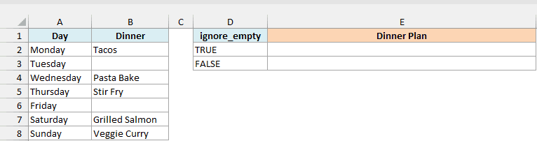
Here is the formula:
=TEXTJOIN(", ",TRUE,B2:B8)
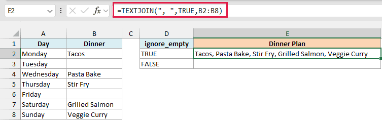
This returns Tacos, Pasta Bake, Stir Fry, Grilled Salmon, Veggie Curry. The two blank cells are skipped entirely.
Now enter the FALSE version in E3.
Here is the formula:
=TEXTJOIN(", ",FALSE,B2:B8)
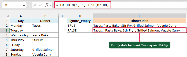
This returns Tacos, , Pasta Bake, Stir Fry, , Grilled Salmon, Veggie Curry.
Each blank dinner keeps its position, so there’s an empty entry between the commas for Tuesday and Friday.
Pro Tip: TRUE skips missing entries, which usually gives you the list you want. Choose FALSE for export lines where every field must keep its position.
TRUE also skips formulas that return "", so those cells leave no gaps in the joined list.
But a cell holding just a space isn’t empty, so TEXTJOIN still includes it in the list.
To remove those spaces before joining, use the TRIM function.
TEXTJOIN vs CONCAT vs CONCATENATE
These three functions all join text, but their options differ:
| Feature | TEXTJOIN | CONCAT | CONCATENATE |
|---|---|---|---|
| Takes a whole range | ✅ | ✅ | ❌ |
| Lets you set a delimiter | ✅ | ❌ | ❌ |
| Skips empty cells | ✅ | ❌ | ❌ |
| Available in | Excel 2019 and later | Excel 2019 and later | Every version (kept for compatibility) |
The CONCAT function accepts a whole range, but joins everything without a separator. Use TEXTJOIN when you need a separator or want to skip blanks.
The older CONCATENATE function needs individual cell references. Keep it for compatibility with older Excel versions.
The & operator works too, but you have to type the separator each time you join another piece.
Example 3: Build a Product Code from Each Row
Those blank-skipping options also work for product codes.
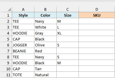
Below are ten products with style, color, and size, and I want to join those parts into SKUs with hyphens in column D.
Some one-size items have no size entered, so their SKUs shouldn’t end with a hyphen.
Here is the formula:
=TEXTJOIN("-",TRUE,A2:C2)
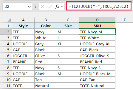
The first result is TEE-Navy-M. For the cap with no size, the result is CAP-Black, because TRUE skips the empty Size cell.
Compare that with =A2&"-"&B2&"-"&C2, copied down. That version always adds both hyphens, so the same cap ends up as CAP-Black-.
TEXTJOIN returns one string per formula, so it doesn’t spill a separate SKU for every row. Enter it in D2 and copy it down to D11.
Pro Tip: In Excel 365, =BYROW(A2:C11,LAMBDA(r,TEXTJOIN("-",TRUE,r))) spills all ten SKUs by running the LAMBDA function once per row.
Example 4: TEXTJOIN with Line Breaks (CHAR 10)
You can also put each item on its own line inside the result cell.
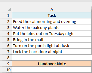
Below is a house-sitting handover list with six tasks, and I want to put each task on a separate line in A10.
Here is the formula:
=TEXTJOIN(CHAR(10),TRUE,A2:A7)
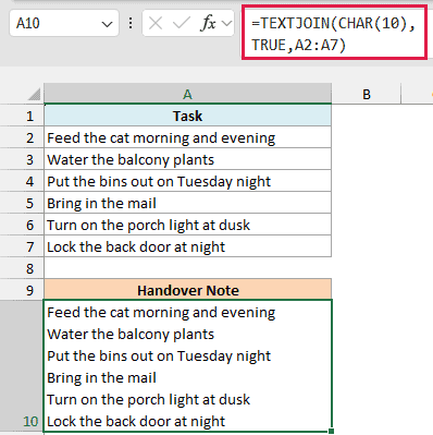
This stacks the six tasks on six lines inside A10. The result cell has Wrap Text turned on and enough row height to show the whole note.
CHAR(10) is the line-break character, also called a line feed. Using it as the delimiter puts a new line between tasks instead of a comma or space.
Important: Without Wrap Text, the tasks in A10 look crammed onto one line. Turn on Wrap Text (Home > Wrap Text) so the line breaks show.
A separate guide shows other ways to start a new line in a cell, including adding a line break manually.
Example 5: Keep Dates and Prices Readable with TEXT
Dates and dollar amounts need a little care when you join them.
Below are three salon bookings with dates and prices, and I want a summary without formatting in F2 and with the TEXT function in F3.

Here is the formula:
=TEXTJOIN(" | ",TRUE,A2:A4&" on "&B2:B4&" ("&C2:C4&")")
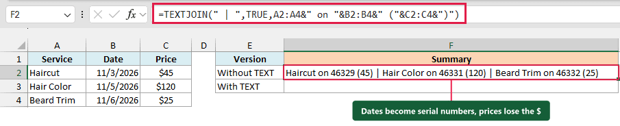
This returns Haircut on 46329 (45) | Hair Color on 46331 (120) | Beard Trim on 46332 (25).
A date is stored as a serial number, and the dollar sign is just part of the cell’s display format. Joining the raw values loses that formatting.
That’s why 11/3/2026 becomes 46329, and $45 becomes 45.
Now enter the version with the TEXT function in F3.
Here is the formula:
=TEXTJOIN(" | ",TRUE,A2:A4&" on "&TEXT(B2:B4,"mmm d")&" ("&TEXT(C2:C4,"$#,##0")&")")

This returns Haircut on Nov 3 ($45) | Hair Color on Nov 5 ($120) | Beard Trim on Nov 6 ($25).
Here is how this formula works:
- The
&operators build a phrase for each row: the service, then the date, then the price in parentheses. Those three phrases form an in-memory array. - The TEXT function locks in the display format before joining.
"mmm d"gives dates such as Nov 3, while"$#,##0"keeps the dollar sign. - TEXTJOIN combines the three phrases with
" | ", a pipe with a space on either side.
Building the array with & works with a normal Enter in Microsoft 365 or Excel 2021 and later. In Excel 2019, confirm these formulas with Ctrl+Shift+Enter.
Example 6: Join Matching Values (TEXTJOIN IF)
You can also join only the entries that match a condition.
Below is a schedule of ten community center classes, and I want to join those matching the day in E1 into one line in E2.
E1 holds Saturday.
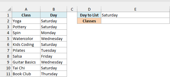
Here is the formula:
=TEXTJOIN(", ",TRUE,FILTER(A2:A11,B2:B11=E1,"No classes"))
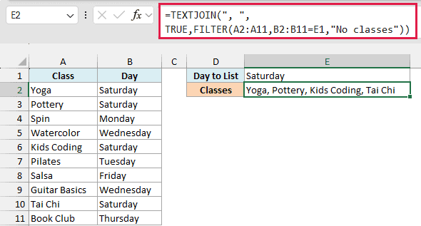
For Saturday, this returns Yoga, Pottery, Kids Coding, Tai Chi.
Here is how this formula works:
- The FILTER function keeps only the classes in A2:A11 where the Day in B2:B11 matches E1.
- FILTER’s third argument,
"No classes", is the message to show when the day has no matching rows. - TEXTJOIN then joins those matched classes into one comma-separated string.
Change the day in E1 and the list updates. A day without classes shows No classes.
FILTER needs Microsoft 365, Excel 2021 or later, or Excel for the web.
If you’re looking for a TEXTJOIN IF formula, this is the same idea: test a condition, then join only the matching values.
In Excel 2019, which doesn’t have the FILTER function, use =TEXTJOIN(", ",TRUE,IF(B2:B11=E1,A2:A11,"")) and confirm with Ctrl+Shift+Enter.
The IF function supplies each matching class and an empty string for every other row, which TEXTJOIN skips because ignore_empty is TRUE.
With Saturday in E1, this returns the same list as the version using the FILTER function.
This also lets you return multiple lookup matches in one cell, instead of stopping at the first match.
Example 7: Join Unique Values Only (Remove Duplicates)
The last example lists each entry just once.
Below are 12 after-school sports sign-ups, and I want to list each sport once, sorted from A to Z, in D2.
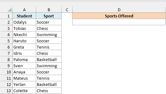
Here is the formula:
=TEXTJOIN(", ",TRUE,SORT(UNIQUE(B2:B13)))
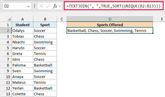
This returns Basketball, Chess, Soccer, Swimming, Tennis.
Here is how this formula works:
- UNIQUE removes the repeated sports from B2:B13, leaving five sports from the 12 sign-ups.
- SORT puts those five sports in A to Z order. Drop SORT if you want to keep their first-seen order instead.
- TEXTJOIN joins that list with a comma and a space between sports.
TEXTJOIN doesn’t remove duplicates by itself. The UNIQUE function removes them before TEXTJOIN joins the values.
The UNIQUE and SORT functions need Microsoft 365 or Excel 2021 and later.
If the repeated items are already together in one cell, see how to remove duplicates from a cell instead.
Start with the range you want to join, choose a separator, and use TRUE when missing entries should disappear from the list.
When the job needs formatting, filtering, or unique values, prepare those values first and let TEXTJOIN combine the result.
I hope you found this article helpful.
Other Excel Articles You May Also Like:
- How to Combine Two Columns in Excel
- CONCATENATE Excel Range (with and without separator)
- TEXTSPLIT Function in Excel
- Text.Combine Function in Power Query M
- Excel VSTACK function
- How to Combine Cells in Excel
- How to Combine First and Last Name in Excel (4 Easy Ways)
- 20 Advanced Excel Functions and Formulas (for Excel Pros)
