PERCENTOF Function in Excel

PERCENTOF is a newer Excel function that works out what percentage a part makes up of a total. You give it the part and the whole, and it does the adding up and the dividing for you.

It’s handy for things like each candidate’s share of the votes, or how much of your sales came from one category. It also works as the calculation inside GROUPBY and PIVOTBY, which is where it saves the most time.

Note that PERCENTOF always returns a single value. So unlike many functions in Microsoft 365, giving it a range won’t spill a separate percentage for every row.

In this article, I’ll show you how to use PERCENTOF with six practical examples, from a simple percentage of total to full percentage summaries with GROUPBY and PIVOTBY.

PERCENTOF Function Syntax

Here is the syntax of the PERCENTOF function:

=PERCENTOF(data_subset, data_all)

• data_subset – The part you want to express as a percentage. It can be a number, a cell, a range, or an array.
• data_all – The whole that the part is compared against. It can also be a number, a cell, a range, or an array.

PERCENTOF adds up everything in data_subset, adds up everything in data_all, and divides the first total by the second. So it works exactly like =SUM(data_subset)/SUM(data_all).

Inside a range, PERCENTOF skips blank cells, text, and TRUE/FALSE values, just like SUM does. So an empty cell or a text note in your data won’t throw off the result.

If either argument contains an error value, such as #N/A, PERCENTOF returns #NUM! instead of passing that error along. So when you see #NUM!, look for an error somewhere in the source data.

The PERCENTOF function works only in Excel for Microsoft 365 (Windows and Mac) and Excel for the web. It’s not available in Excel 2024, 2021, or older versions.

When to Use the PERCENTOF Function

Use this function when you need to:

• Show each item’s share of a total, like votes, sales, or expenses
• Find what percentage a group of values makes up of the whole
• Track how close you are to a goal or target
• Get the share of the total for only the items that meet a condition
• Build percentage summaries by category with GROUPBY and PIVOTBY

Let me show you a few practical examples of how to use the PERCENTOF function.

Example 1: Calculate Percentage of Total With PERCENTOF

Let’s start with a simple example.

Below are the vote counts for six candidates in a class election, and I want to get each candidate’s share of the votes in column C.

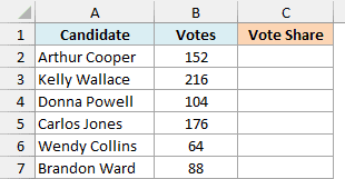
Here is the formula:

=PERCENTOF(B2,$B$2:$B$7)

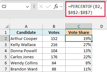
Enter it in C2 and copy it down to C7. Arthur Cooper’s 152 votes out of 800 come to 19%, and Kelly Wallace leads with 27%.

In the above formula, B2 is the part (one candidate’s votes) and $B$2:$B$7 is the whole.

The dollar signs make the total range an absolute reference, so it stays the same as you copy the formula down, while B2 changes to B3, B4, and so on.

PERCENTOF returns a decimal, so I’ve formatted column C as a percentage. Without that formatting, you’d see 0.19 instead of 19%.

Important: Don’t give PERCENTOF a range in both arguments expecting a percentage for each row. A formula like =PERCENTOF(B2:B7,B2:B7) adds up both ranges and returns a single 100%, so you need one formula per row.

If you’re using Excel 2024 or an older version, enter the below formula in cell C2 and then copy it down the range:

=B2/SUM($B$2:$B$7)

Example 2: Find the Share of Several Values Combined

Here’s another practical scenario.

Below is a reading log with the pages read on each day of a week, and I want to find what share of the week’s pages were read on the weekend, in cell E2.

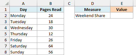
Here is the formula:

=PERCENTOF(B7:B8,B2:B8)

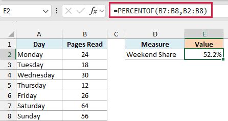
This returns 52.2%, so more than half of the week’s reading happened on Saturday and Sunday.

Here, data_subset is the range B7:B8 (Saturday and Sunday). PERCENTOF adds those two days (64 + 56 = 120) and divides that by the total for all seven days, which is 230.

You might reach for =SUM(B7:B8)/SUM(B2:B8) here, and that works too. PERCENTOF does that adding for you, so the formula stays shorter and easier to read.

Pro Tip: If the cells you want aren’t next to each other, put them inside an extra pair of parentheses, separated by a comma. For example, =PERCENTOF((B2,B4),B2:B8) gives the share of pages read on Monday and Wednesday (23.5%).

Example 3: Track Progress Toward a Goal

Now let’s look at something a bit different.

Below are the amounts collected by eight volunteers for a charity fundraiser, and I want to find what percentage of the $5,000 goal in E2 they’ve reached so far, in cell E3.

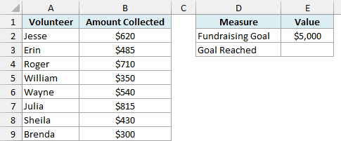
Here is the formula:

=PERCENTOF(B2:B9,E2)

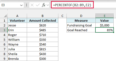
This returns 85%, since the volunteers have collected $4,250 of the $5,000 goal.

Here, data_all isn’t a list of values but a single target in E2. The part doesn’t have to be inside the whole, since PERCENTOF only compares the two totals.

This also means the result can go past 100%. If the volunteers end up collecting $5,600, the formula returns 112%, which is exactly what you’d want to see when a goal is beaten.

If the goal cell is empty, PERCENTOF returns the #DIV/0! error, as there’s nothing to divide by.

Example 4: Get the Percentage of Total for One Category

Let’s step it up and combine PERCENTOF with the FILTER function.

Below are a coffee shop’s weekly sales by item, and I want to find what share of the total sales comes from the category in F2 (Bakery), in cell F3.

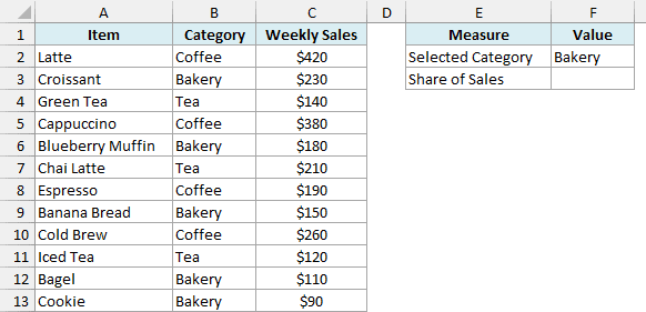
Here is the formula:

=PERCENTOF(FILTER(C2:C13,B2:B13=F2),C2:C13)

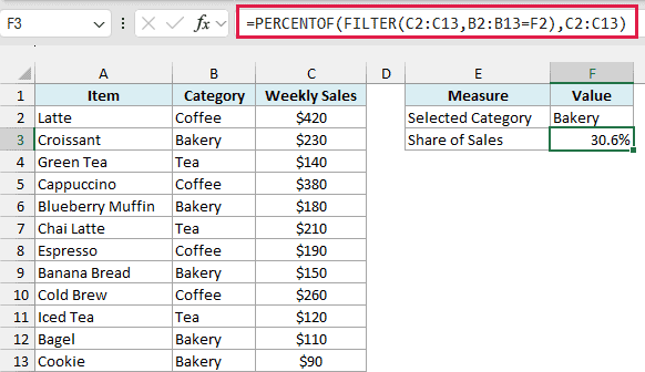
This returns 30.6%, so bakery items bring in a little under a third of the week’s sales.

How this formula works:

• FILTER(C2:C13,B2:B13=F2) pulls out the sales of every item whose category matches F2. That’s 230, 180, 150, 110, and 90.
• PERCENTOF adds those up (760) and divides by the total of all the sales in C2:C13, which is 2,480.

Since the category comes from F2, you can change it to Coffee or Tea, and the share updates on its own. Coffee comes to 50.4% and Tea to 19.0%.

Important: If F2 has a category that isn’t in the list, FILTER finds nothing and the formula returns the #CALC! error. To get 0% instead, add 0 as FILTER’s third argument: =PERCENTOF(FILTER(C2:C13,B2:B13=F2,0),C2:C13).

Example 5: PERCENTOF With GROUPBY (Percentage of Total by Category)

Now let’s use PERCENTOF to build a whole summary with one formula. The GROUPBY function summarizes data by category, and PERCENTOF can be the calculation it runs.

Below are the expenses from a four-day trip, and I want a summary of each category’s share of the total trip cost in columns E and F.

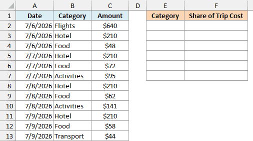
Here is the formula:

=GROUPBY(B2:B13,C2:C13,PERCENTOF,,,-2)

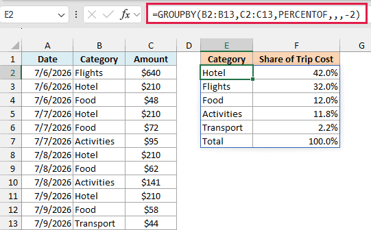
This gives one row for each category with its share of the trip cost, plus a Total row of 100%. The hotel took the biggest chunk at 42.0%, followed by the flights at 32.0%.

How this formula works:

• B2:B13 is the column to group by (the category).
• C2:C13 holds the values to calculate (the amounts).
• PERCENTOF is the calculation. It’s written without parentheses, and GROUPBY gives it each category’s amounts as the part and all the amounts as the whole.
• -2 is the sort_order argument. It sorts by the second column (the share) from largest to smallest, and the two empty arguments before it skip field_headers and total_depth.

Since the ranges have no header row, GROUPBY doesn’t return one either, so I’ve typed the headers into E1:F1.

Example 6: PERCENTOF With PIVOTBY (Percentage of Row Total)

Let’s finish with a two-way summary using the PIVOTBY function.

Below are the tickets sold for four movies over a weekend, and I want to see what share of each movie’s tickets sold on each day, starting in cell E1.

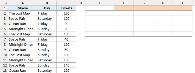
Here is the formula:

=PIVOTBY(A2:A13,B2:B13,C2:C13,PERCENTOF,,,,,,,1)

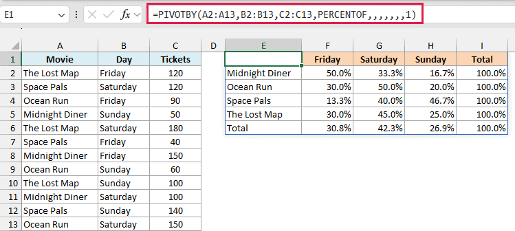
This creates a grid with the movies down the side and the days across the top. Midnight Diner sold half of its tickets on Friday, while Space Pals did best on Sunday with 46.7%.

How this formula works:

• A2:A13 (the movies) become the rows, and B2:B13 (the days) become the columns.
• C2:C13 holds the ticket counts, and PERCENTOF turns each count into a share.
• 1 is the last argument, relative_to. It tells PIVOTBY to divide by each row’s total, which is why the Total column shows 100% for every movie.

If you leave relative_to out (or use 0), each day column adds up to 100% instead, which shows how each day’s tickets split across the movies. Use 2, and every cell becomes a share of all 1,300 tickets.

The Total row at the bottom shows how all the tickets split across the weekend: 30.8% on Friday, 42.3% on Saturday, and 26.9% on Sunday.

So these are six ways to use the PERCENTOF function in Excel, from a simple percentage of total to percentage summaries with GROUPBY and PIVOTBY.

I hope you found this Excel tutorial useful.

List of All Excel Functions

Other Excel Articles You May Also Like:

• How to Calculate Percentage Change in Excel
• SUMIF Function in Excel
• PERCENTRANK Function in Excel
• PERCENTILE.INC Function in Excel
• PERCENTILE.EXC Function in Excel