

The PERCENTRANK.INC function tells you where a number stands within a list by returning its percentile rank. A higher result means the number sits farther up the list, which helps you compare amounts, prices, or measurements on the same scale.
It can also rank a number that falls between two values in your data. I’ll show you how that works, how to get ranks for a whole column, and why repeated values and the precision setting deserve a closer look.
Follow along with the example file
PERCENTRANK.INC Function Examples.xlsx
PERCENTRANK.INC Function Syntax
Here is the syntax of the PERCENTRANK.INC function:
=PERCENTRANK.INC(array,x,[significance])
- array is the numeric dataset you want to compare against. You can give it a cell range, and the values don’t need to be sorted.
- x is the number you want to rank. In Excel versions with dynamic arrays, you can also give it a range of numbers to get one result for each.
- significance is optional and controls the precision of the returned decimal. If you leave it out, Excel keeps three digits after the decimal point, such as 0.555.
The significance setting changes the value Excel calculates, not just how the cell looks. A larger setting keeps more digits, as you’ll see in Example 3; a setting below 1 gives a #NUM! error.
PERCENTRANK.INC works in Excel 2010 and later. The spilling examples below require Microsoft 365, Excel 2021 or 2024, or Excel for the web.
When to Use the PERCENTRANK.INC Function
Use this function when you need to:
- See whether a bill or price is near the low or high end of a list.
- Compare a proposed number with an existing set of values.
- Put measurements on a percentile scale so their relative positions are easier to compare.
Let me show you how this works with a few examples from the downloadable workbook.
Example 1: Rank a Whole List of Bills
Let’s start by getting a percentile rank for every amount in one go.
Below is a list of cafe bills, and I want to show each amount’s percentile rank in column C so we can compare it with the other bills.
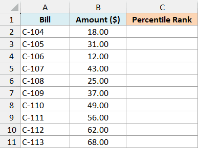
Enter this formula in cell C2 on the Cafe Bills sheet:
=PERCENTRANK.INC(B2:B11,B2:B11)
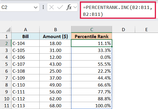
The first B2:B11 is the list we compare against. The second B2:B11 asks Excel to rank each amount in that list, so the results spill down from C2 automatically.
The result cells in the workbook use Percentage format with one decimal place. For example, the formula returns 0.111 for the $18 bill, and the cell displays 11.1%.
The smallest bill, $12, returns 0%, and the largest, $68, returns 100%. These amounts are all different, so Excel spreads their positions across nine equal intervals, one fewer than the ten bills.
The $43 bill has five smaller amounts. Its rank is 5 divided by 9, which the default precision reduces to 0.555, displayed as 55.5%.
That is a percentile position, not the percentage of the ten bills below $43. Five out of ten bills are below it, which would be 50%, a different calculation.
Important: Make sure the cells below C2 are empty before entering the spilling formula. If something blocks the result area, Excel returns a #SPILL! error.
If you are using Excel 2019 or earlier, enter the below formula in cell C2 and then copy it down to C11:
=PERCENTRANK.INC($B$2:$B$11,B2)
The dollar signs keep the comparison range fixed as you copy down. The B2 reference changes to B3, B4, and so on, so each bill gets its own rank.
Example 2: Rank Prices Between Existing Values
The number you want to rank doesn’t have to appear in the list.
Below are ticket prices for ten venues, and I want to compare four proposed prices with them and show the percentile ranks in column E.
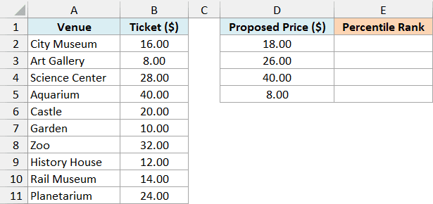
Enter this formula in cell E2 on the Ticket Prices sheet:
=PERCENTRANK.INC(B2:B11,D2:D5)
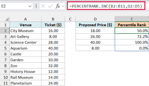
Here, B2:B11 is the existing price list, while D2:D5 contains the four prices we want to check. The results spill into E2:E5: 50.0%, 72.2%, 100.0%, and 0.0%.
The proposed price of $18 isn’t in the list. It sits halfway between $16 and $20, so Excel calculates a rank halfway between their percentile positions, giving 50%.
This is called interpolation. The size of the gap between the two prices matters, so a value closer to $16 would get a rank closer to $16’s position.
Notice that the proposed prices stay outside the comparison list. Adding them to the original list would change the dataset and could change the ranks you’re trying to measure.
Important: Interpolation only works within the dataset’s range. If you change a proposed price to below $8 or above $40, PERCENTRANK.INC returns #N/A instead of estimating beyond the endpoints.
Example 3: Keep More Digits in the Result
Sometimes changing the cell format isn’t enough to show the precision you need.
Below is a list of book lengths, and I want to find the percentile rank of the 320-page target in D2, first in E2 and then with more precision in F2.
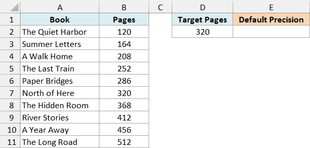
Enter this formula in cell E2 on the Book Lengths sheet:
=PERCENTRANK.INC(B2:B11,D2)
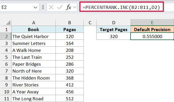
This returns 0.555. The cell is formatted to show six decimal places, so you see 0.555000, but those extra zeros don’t add any precision.
To keep six digits in the calculation, enter this formula in F2:
=PERCENTRANK.INC(B2:B11,D2,6)
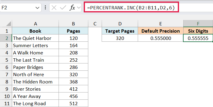
This returns 0.555555. Both cells use the same number format, so the difference comes from the significance argument.
There are five shorter books in this ten-book list, giving a rank of 5 divided by 9. That fraction repeats, and PERCENTRANK.INC truncates the extra digits rather than rounding them up.
If a later formula uses this rank, it uses the stored value. Increase significance when those extra digits matter; adding decimal places through formatting cannot recover digits the function discarded.
Follow along with the example file
PERCENTRANK.INC Function Examples.xlsx
Example 4: Understand Ties in Percentile Ranks
Repeated values get the same percentile rank, including repeated values at the top of the list.
Below are distances from ten walks, and I want to show each walk’s percentile rank in column C, including the distances that appear twice.
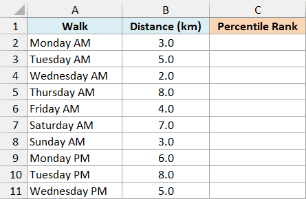
Enter this formula in cell C2 on the Walk Distances sheet:
=PERCENTRANK.INC(B2:B11,B2:B11)
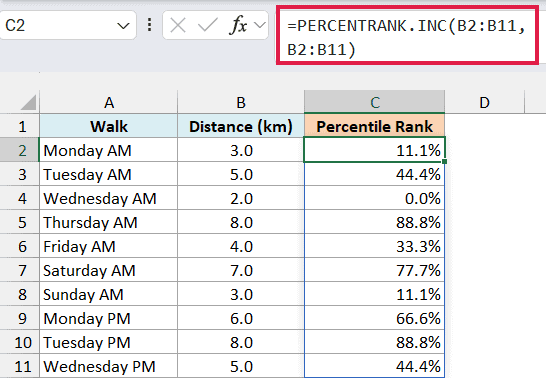
Both 3 km walks return 11.1%, and both 5 km walks return 44.4%. Excel gives tied values the position of their first occurrence when the numbers are arranged from smallest to largest.
For the 5 km walks, four distances are smaller: 2, 3, 3, and 4. Dividing four by nine gives 0.444 after truncation, which displays as 44.4%.
The two 8 km walks are the largest, but both return 88.8%. Eight distances are smaller, so their rank is 8 divided by 9, not 1.
Important: Don’t assume the largest value always returns 100%. A repeated maximum can return less than 100%, as the two 8 km walks show here.
The original row order doesn’t break the tie. Sorting the same distances won’t turn one of the 8 km walks into a 100% result.
Example 5: Compare PERCENTRANK.INC and PERCENTRANK.EXC
The INC and EXC versions use different percentile scales, so the same number can get different ranks.
Below are nine movie runtimes, and I want to compare their inclusive ranks in column C with their exclusive ranks in column D.
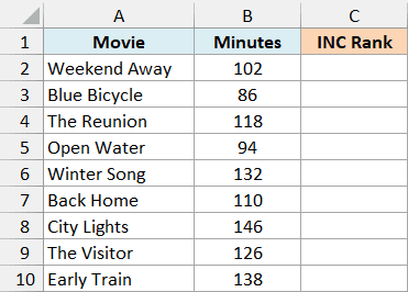
First, enter this formula in cell C2 on the Movie Runtimes sheet:
=PERCENTRANK.INC(B2:B10,B2:B10)
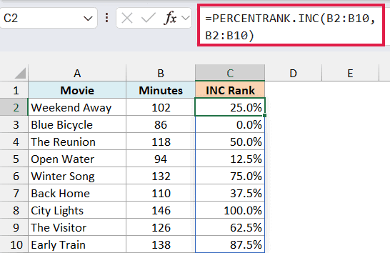
These runtimes are all different. INC assigns 0% to the shortest, 86 minutes, and 100% to the longest, 146 minutes, with 12.5 percentage points between each sorted position.
Now enter the EXC version in cell D2:
=PERCENTRANK.EXC(B2:B10,B2:B10)
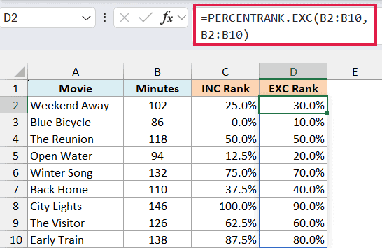
EXC returns 10% for the shortest movie and 90% for the longest. Its positions are spaced by 1 divided by 10, or 10 percentage points, because its denominator is one more than the nine values.
Both methods put the middle runtime, 118 minutes, at 50%. Away from the middle, their results differ, so use the method your report or analysis calls for consistently.
Neither function removes the smallest or largest value from the data. The difference is how it assigns percentile positions to those values.
The older PERCENTRANK function uses the inclusive convention and remains available for compatibility. For a new workbook using that convention, PERCENTRANK.INC makes the choice explicit.
If you already have a percentile, such as 75%, and want the corresponding runtime instead, use the PERCENTILE.INC function. It takes the percentile as input and returns a value from the distribution.
So these are a few ways to use PERCENTRANK.INC to compare numbers, interpolate between them, and control precision. I hope you found this tutorial helpful.
Other Excel Articles You May Also Like:
