

The DOLLARFR function in Excel converts a decimal number into a fractional dollar number. The digits after the decimal point become the top of a fraction, so 1.125 in sixteenths turns into 1.02, which you read as 1 and 2/16.
It comes from the days when stock prices were quoted in eighths and sixteenths of a dollar. US Treasury prices are still quoted in 32nds, and the same idea works for anything you measure in fractions, like inches or baseball innings.
There’s one catch, though. DOLLARFR expects one number at a time, so pointing it at a whole range returns a #VALUE! error.
In Microsoft 365, Excel 2024, and Excel 2021, a plus sign in front of the range fixes this (I’ll show you how in the first example).
In this tutorial, I’ll show you how to read DOLLARFR results, use different fractions, build bond quotes, round measurements first, and avoid the errors it can return.
Follow along with the example file
DOLLARFR Function Examples.xlsx
DOLLARFR Function Syntax
Here is the syntax of the DOLLARFR function:
=DOLLARFR(decimal_dollar, fraction)
- decimal_dollar is the decimal number you want to convert, such as a price of 24.5625.
- fraction is the whole number to use as the bottom of the fraction, such as 8, 16, or 32.
The fraction also decides how many digits you get after the decimal point.
A fraction from 2 to 10 gives one digit, so 1.1 in eighths means 1 and 1/8. A fraction from 11 to 100, such as 16 or 32, gives two, so 1.02 in sixteenths means 1 and 2/16.
The DOLLARFR function works in Microsoft 365, Excel 2024, Excel 2021, Excel 2019, Excel 2016, and Excel for Mac.
When to Use the DOLLARFR Function
Use this function when you need to:
- Show decimal stock or bond prices in eighths, sixteenths, or 32nds.
- Turn Treasury prices into the dash quotes traders use, like 99-16.
- Show any measurement that’s counted in fractions, like drill bit sizes in 64ths or innings pitched in thirds.
Let me show you a few practical examples of how to use DOLLARFR.
Example 1: Convert Decimal Prices to Sixteenths
Let’s start with a simple example.
Below is a list of share prices in decimals, and I want to show each one in sixteenths in column C.
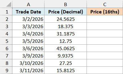
In Microsoft 365, Excel 2024, or Excel 2021, enter this formula in cell C2 and press Enter:
=DOLLARFR(+B2:B9,16)
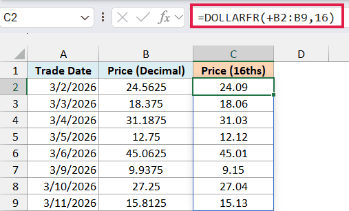
The above formula converts every price in B2:B9 to sixteenths, and the results spill into C2:C9. You only enter it once.
To read a result, keep the whole number as it is and treat the digits after the decimal point as sixteenths. So 24.09 means 24 and 9/16, which is the same as 24.5625.
The plus sign in front of B2:B9 matters. Without it, =DOLLARFR(B2:B9,16) returns a single #VALUE! error instead of eight results.
That’s because DOLLARFR is an older function that expects one number and won’t accept a range reference. The plus sign turns the range into a list of values, and DOLLARFR then converts each one.
If you’re using Excel 2019 or earlier, enter the below formula in cell C2 and then copy it down to C9:
=DOLLARFR(B2,16)
The same goes for the later examples that return one column of results. Point the formula at the first cell of each range, then copy it down.
Important: Excel sees 24.09 as just 24.09, not 24.5625, so adding or averaging the results in column C gives wrong answers. Do your math on the decimal prices in column B, and use DOLLARFR only to show the final result.
Example 2: Show the Same Size in Different Fractions
Now let’s see how the fraction argument changes the result.
Below is a list of drill bit sizes in inches, and I want to show each size in eighths, sixteenths, 32nds, and 64ths in columns B to E.
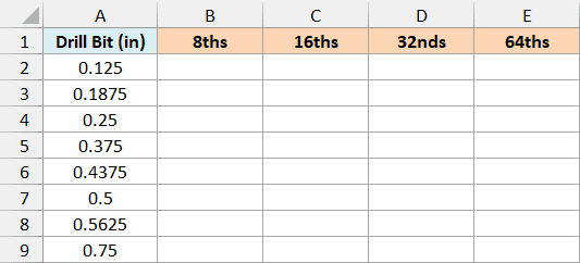
Enter the following formula in cell B2:
=DOLLARFR(+A2:A9,{8,16,32,64})
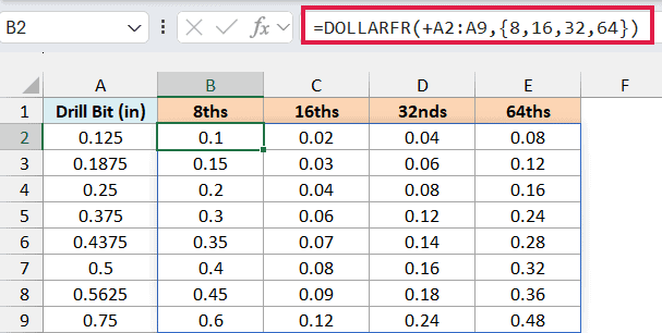
The {8,16,32,64} part is a list of four fractions. DOLLARFR uses each of them with every size, so this one formula fills all eight rows and all four columns.
If you’re using Excel 2019 or earlier, enter the below formula in cell B2, copy it down to B9, and then do the same in columns C, D, and E with 16, 32, and 64:
=DOLLARFR(A2,8)
Look at how many digits each column has. Eighths get one digit after the decimal point (0.3 is 3/8), while 16ths, 32nds, and 64ths get two (0.06 is 6/16).
But check 0.1875 in eighths. It returns 0.15, which doesn’t mean 15/8.
The size 0.1875 is 1.5 eighths, and DOLLARFR shows the 1.5 as the digits 15.
So whenever you see an extra digit like that, the value doesn’t fit that fraction exactly. 0.1875 is 3/16 of an inch, and the 16ths, 32nds, and 64ths columns show it cleanly as 0.03, 0.06, and 0.12.
Also, DOLLARFR doesn’t simplify the fraction. Half an inch shows as 0.08 in sixteenths, which is 8/16, not 1/2.
Example 3: Convert Treasury Bond Prices to 32nds
US Treasury notes and bonds are still quoted in 32nds, and that’s where DOLLARFR comes in handy.
Below is a list of Treasury prices in decimals, and I want to show them in 32nds in column C and as dash quotes in column D.
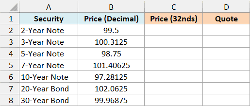
Enter the following formula in cell C2:
=DOLLARFR(+B2:B8,32)
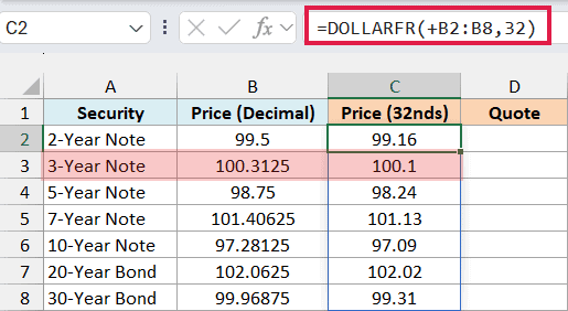
This converts each price to 32nds. For example, 99.16 means 99 and 16/32, which is the 99.5 in column B.
Now look at the 3-Year Note. Its result shows 100.1, but that doesn’t mean 1/32.
The price 100.3125 is 100 and 10/32, so the result is really 100.10, and Excel drops the trailing zero.
That’s easy to misread. You can fix it by formatting column C to show two decimal places, or by turning the results into the dash quotes that bond traders use, like 99-16.
To get the dash quotes, enter this formula in cell D2:
=SUBSTITUTE(TEXT(DOLLARFR(+B2:B8,32),"0.00"),".","-")
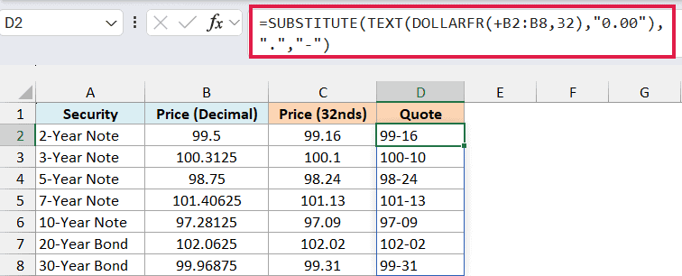
How this formula works:
DOLLARFR(+B2:B8,32)converts each price to 32nds, the same as column C.- The TEXT function turns each result into text with exactly two decimal places, so 100.1 becomes 100.10.
- The SUBSTITUTE function replaces the decimal point with a dash, which gives you 100-10.
The quotes in column D are text, so they’re only for display. Keep the decimal prices in column B for any calculations.
Example 4: Show Innings Pitched From Outs
DOLLARFR isn’t only for prices. It works with anything that’s counted in fractions, and baseball innings are a good example.
Each inning has three outs, so innings pitched are written as 6.1 or 6.2, which means 6 and 1/3 or 6 and 2/3 innings.
Below is a list of pitchers with the number of outs each one recorded, and I want to show their innings pitched in column C.
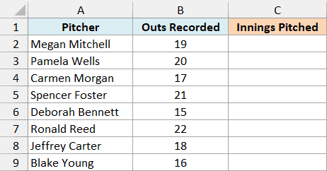
Enter the following formula in cell C2:
=DOLLARFR(B2:B9/3,3)
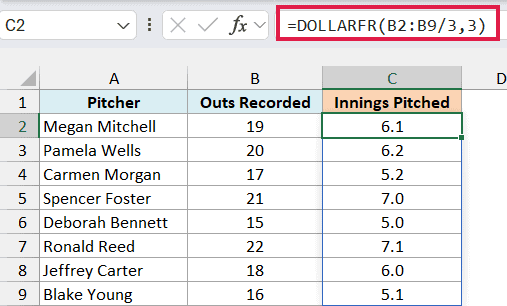
Here, B2:B9/3 turns the outs into innings, so 19 outs becomes 6.333 innings. DOLLARFR then shows the 0.333 part in thirds, which gives you 6.1.
This time, there’s no plus sign in front of the range. B2:B9/3 is already a calculation that returns a list of values, so DOLLARFR accepts it as it is.
The example file formats column C to show one decimal place, so full innings show the box-score way, such as 7.0 for 21 outs. In your own sheet, apply the 0.0 number format to column C to get the same look.
Example 5: Round to the Nearest 1/16 Before Converting
Here’s a problem you’ll run into with real measurements.
Below is a cut list for a bookshelf with lengths in decimal inches, and I want to show each length in sixteenths of an inch, first without rounding in column C and then rounded to the nearest 1/16 in column D.
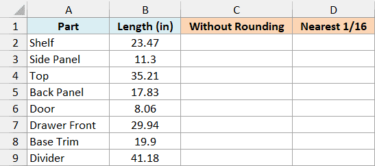
First, let’s see what DOLLARFR does on its own. Enter the following formula in cell C2:
=DOLLARFR(+B2:B9,16)
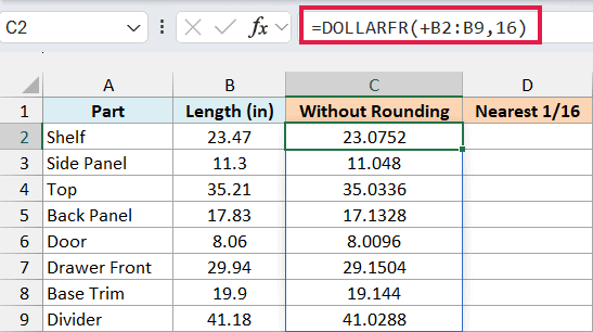
The results have extra digits, like 23.0752 for the shelf. That’s because 23.47 inches isn’t a whole number of sixteenths (0.47 inches is 7.52/16), and DOLLARFR shows the leftover as more digits.
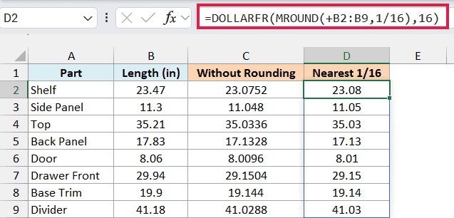
You can’t mark 7.52/16 on a tape measure, so you need to round each length to the nearest 1/16 first. Enter this formula in cell D2:
=DOLLARFR(MROUND(+B2:B9,1/16),16)
How this formula works:
- The MROUND function rounds each length to the nearest multiple of 1/16, so 23.47 becomes 23.5.
- MROUND has the same quirk as DOLLARFR and returns #VALUE! with a plain range, so it needs the plus sign in front of B2:B9 too.
- DOLLARFR then shows 23.5 in sixteenths as 23.08, which is 23 and 8/16.
If you work to a different precision, change both numbers. For the nearest 1/8 inch, use 1/8 inside MROUND and 8 in DOLLARFR.
If you’d rather see the lengths as real fractions like 23 1/2 while keeping the actual value in the cell, a fraction number format is the better choice. Here’s how to show numbers as fractions in Excel.
Example 6: Why DOLLARFR Returns #DIV/0!, #NUM!, or #VALUE!
Finally, let’s look at what DOLLARFR does with unusual inputs, so an error doesn’t catch you off guard.
Below is a set of test cases with a price and a fraction in each row, and I want to see what DOLLARFR returns for each one in column D.
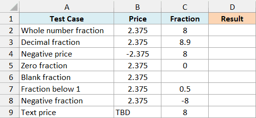
Enter the following formula in cell D2:
=DOLLARFR(+B2:B9,+C2:C9)
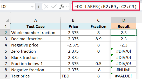
Both ranges have a plus sign this time, because both arguments come from a range.
The first row is the normal case. 2.375 in eighths returns 2.3, which means 2 and 3/8.
The second row uses 8.9 as the fraction, and it returns the same 2.3. DOLLARFR drops the decimal part of the fraction, the way the TRUNC function does, so 8.9 works like 8 (it doesn’t round up to 9).
The negative price in the third row works fine. -2.375 returns -2.3, and the minus sign stays.
A fraction of 0 returns #DIV/0!. The blank fraction cell counts as 0, so it returns #DIV/0! too.
The fraction 0.5 also returns #DIV/0!. DOLLARFR drops the decimal part, which leaves 0, so make sure your fraction is at least 1.
A negative fraction returns #NUM!, and the text TBD in the price column returns #VALUE! because it isn’t a number.
So these are a few ways to use the DOLLARFR function in Excel. Just remember to put a plus sign in front of a range, and do your math on the decimal values, not on the DOLLARFR results.
To go the other way, from 24.09 back to 24.5625, Excel has the DOLLARDE function.
And despite the name, DOLLARFR doesn’t add a dollar sign. If you want a number shown as currency text, use the DOLLAR function.
I hope you found this tutorial useful.
Other Excel Articles You May Also Like:
