

The DOLLARDE function in Excel converts a price written in fractional notation, such as 45.3 for 45 and 3/8 of a dollar, into a regular decimal number. It was made for stock and bond prices quoted in eighths, sixteenths, or thirty-seconds.
It also works on anything typed with a dot between two units, like 7.45 for 7 hours and 45 minutes, or 5.11 for 5 feet 11 inches.
You tell DOLLARDE the bottom of the fraction, and it uses that to decide how many digits after the dot to read. So with minutes, 7.5 is read as 7 hours and 50 minutes, not 7 hours and 5 minutes.
Also, DOLLARDE doesn’t accept a range of cells directly, even in Microsoft 365. I’ll show you the small fix for that in Example 2.
Below, I’ll show you how to use DOLLARDE with stock prices, timesheets, heights, and bond quotes, and how to spot entries like 3.75 (75 minutes) that DOLLARDE converts without any error.
Follow along with the example file
DOLLARDE Function Examples.xlsx
DOLLARDE Function Syntax
Here is the syntax of the DOLLARDE function:
=DOLLARDE(fractional_dollar, fraction)
- fractional_dollar is the number in fractional notation. The part before the decimal point is the whole number, and the digits after it are the numerator of the fraction. This argument is required.
- fraction is the denominator of the fraction, such as 8 for eighths, 16 for sixteenths, or 32 for thirty-seconds. This argument is also required.
DOLLARDE reads as many digits after the decimal point as the biggest possible numerator has. With 8, the numerator can only go up to 7, so it reads one digit and 45.3 means 45 and 3/8.
With 16, 32, or 60, the numerator can go up to 15, 31, or 59, so DOLLARDE reads two digits. With 16, 1.1 is read as 1.10, which means 1 and 10/16, not 1 and 1/16.
If the fraction isn’t a whole number, DOLLARDE drops the decimal part, so 16.9 works the same as 16. That’s why anything from 0 up to (but not including) 1 returns #DIV/0!, because it becomes 0 and DOLLARDE divides by zero.
You get the same #DIV/0! error when the fraction points to an empty cell. A fraction below 0 returns the #NUM! error.
The DOLLARDE function works in Microsoft 365, Excel 2024, Excel 2021, Excel 2019, and Excel 2016, on both Windows and Mac. The formulas in this tutorial that fill several cells at once need Microsoft 365, Excel 2024, or Excel 2021.
When to Use the DOLLARDE Function
Use this function when you need to:
- Convert stock or bond prices quoted in fractions, like 1/8 or 1/32 of a dollar, into decimal prices.
- Turn hours and minutes typed as h.mm (7.45 for 7 hours and 45 minutes) into decimal hours.
- Convert measurements typed as feet.inches into one number you can calculate with.
Let me show you a few practical examples of how to use DOLLARDE.
Example 1: Convert Fractional Stock Prices to Decimals
Let’s start with a simple example.
Below is a list of stock prices quoted in eighths of a dollar, where 45.3 means 45 and 3/8, and I want the decimal price of each one in column C.
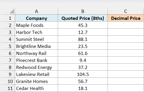
Here is the formula, entered in cell C2 and copied down to C11:
=DOLLARDE(B2,8)
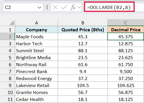
The 8 tells DOLLARDE that the prices are in eighths. For 45.3, it takes the 3 after the decimal point, divides it by 8 to get 0.375, and adds that to 45, so the result is 45.375.
The numerator of an eighth only goes up to 7, so DOLLARDE reads just one digit after the decimal point. That’s all these prices need.
I’ve kept this as one formula per row so you can see how DOLLARDE handles a single price. In the next example, I’ll show you how to convert a whole column with one formula.
Example 2: Convert Hours and Minutes to Decimal Hours
Here’s a use you’re more likely to run into than stock prices.
Below is a timesheet where the hours are typed as h.mm, so 7.45 means 7 hours and 45 minutes, and I want the decimal hours for each employee in column C.
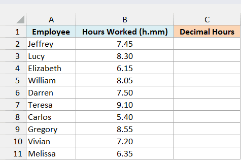
Here is the formula:
=DOLLARDE(+B2:B11,60)
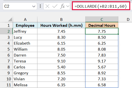
An hour has 60 minutes, so 60 is the fraction. DOLLARDE turns 7.45 into 7 plus 45/60, which is 7.75 hours, and the results spill down from C2.
The minutes can go up to 59, so DOLLARDE reads two digits after the decimal point. That means 8.30 is 8 hours and 30 minutes, and it becomes 8.50.
The plus sign in front of B2:B11 is the important part. To show you why, I’ve entered the same formula without the plus sign in cell E2:
=DOLLARDE(B2:B11,60)
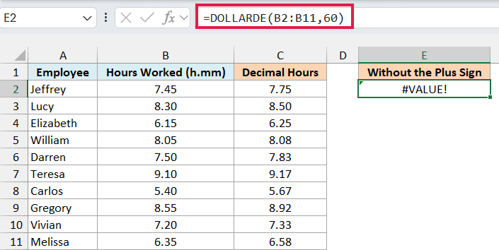
Instead of ten results, you get a single #VALUE! error. Like the EOMONTH function and a few other older functions, DOLLARDE doesn’t accept a range of cells as its input, even in Microsoft 365.
The plus sign turns the range into a list of values, which DOLLARDE can work with, so it returns one result for each row. You can read more about this trick in my article on Excel functions that won’t spill.
A double minus (--B2:B11) or multiplying by 1 (B2:B11*1) would also work. The plus sign is just the shortest way to do it.
Using DOLLARDE for hours only makes sense when the hours are typed as plain numbers like 7.45. If your timesheet holds real Excel times like 7:45, you don’t need DOLLARDE, and you can convert time to decimal by multiplying it by 24.
Important: For less than 10 minutes, type a zero before the minutes. 8.05 is 8 hours and 5 minutes (8.08), but 8.5 is read as 8 hours and 50 minutes, which returns 8.83.
Excel stores 7.5 and 7.50 as the same number, so DOLLARDE always reads them as 7 hours and 50 minutes. If someone worked 7 hours and 5 minutes, the entry has to be 7.05.
If you are using Excel 2019 or earlier, enter the below formula in cell C2 and then copy it down to C11:
=DOLLARDE(B2,60)
Example 3: Convert Heights in Feet and Inches to Centimeters
Now let’s use a different fraction.
Below is a list of student heights typed as feet.inches, where 5.11 means 5 feet 11 inches, and I want each height in centimeters in column C.
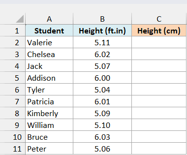
Here is the formula:
=DOLLARDE(+B2:B11,12)*30.48
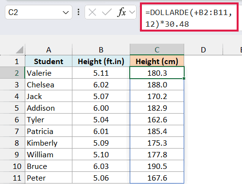
A foot has 12 inches, so 12 is the fraction. DOLLARDE turns 5.11 into 5 plus 11/12, which is about 5.917 feet, and multiplying by 30.48 (the number of centimeters in a foot) gives 180.3 cm.
The same leading-zero rule from Example 2 applies here. William’s 5.10 is 5 feet 10 inches (177.8 cm), so a height of 5 feet 1 inch has to be typed as 5.01.
If you want the height in inches instead, multiply by 12 rather than 30.48. You could also use the CONVERT function, as in =CONVERT(DOLLARDE(+B2:B11,12),"ft","cm"), which gives the same results.
If you are using Excel 2019 or earlier, enter the below formula in cell C2 and then copy it down to C11:
=DOLLARDE(B2,12)*30.48
Example 4: Convert Bond Quotes Like 99-16 to Decimal Prices
Let’s step it up with a case where the data isn’t in the format DOLLARDE expects.
Below are daily quotes for a US Treasury bond copied from a website as text, where 99-16 means 99 and 16/32 of a dollar, and I want the decimal price in column C.
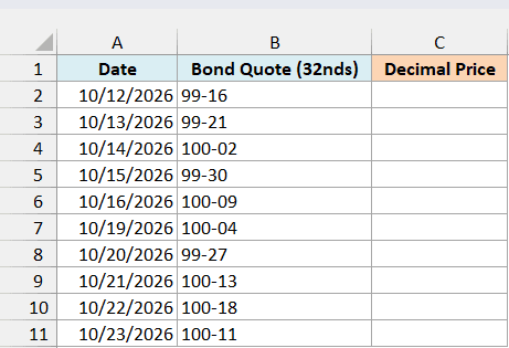
Treasury bond prices are quoted in 32nds, and they’re usually written with a dash instead of a decimal point. If you give “99-16” to DOLLARDE as it is, you get a #VALUE! error.
Here is the formula:
=DOLLARDE(SUBSTITUTE(B2:B11,"-","."),32)
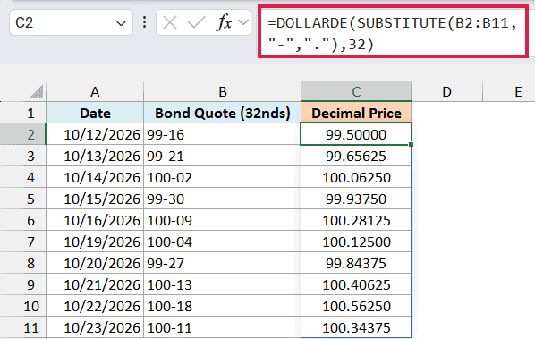
How this formula works:
- The SUBSTITUTE function replaces the dash with a dot, so “99-16” becomes “99.16”.
- DOLLARDE reads 99.16 as 99 and 16/32, and returns 99.5. It accepts the text because “99.16” looks like a number.
- There’s no plus sign here because the SUBSTITUTE function already hands DOLLARDE a list of values, not a range.
For 100-02, you get 100.0625, because 2/32 is 0.0625. The quotes always have two digits after the dash, so the leading-zero problem from Example 2 doesn’t come up here.
If you are using Excel 2019 or earlier, enter the below formula in cell C2 and then copy it down to C11:
=DOLLARDE(SUBSTITUTE(B2,"-","."),32)
Example 5: Flag Entries Where the Fraction Is Too Big
Here’s one more thing to watch out for.
Below is a task log with the time spent on each task typed as h.mm, and I want the decimal hours in column C and a checked version in column D that flags entries with 60 or more minutes.
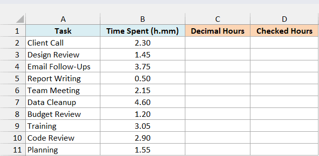
Here is the formula for column C:
=DOLLARDE(+B2:B11,60)
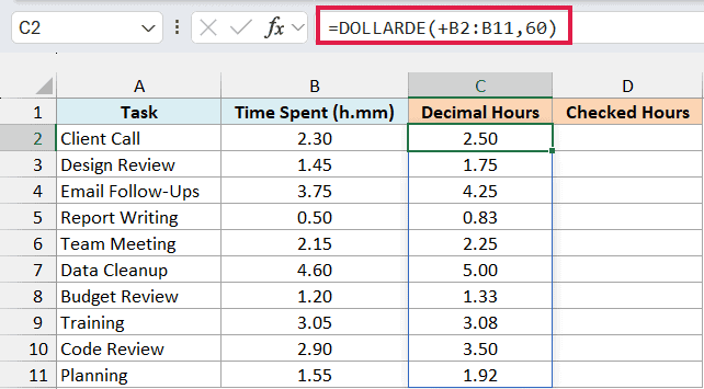
Look at 3.75 for Email Follow-Ups. There’s no such thing as 75 minutes past the hour, so this entry is most likely a typo, but DOLLARDE doesn’t complain.
It simply adds 75/60 to 3 and returns 4.25. The same happens with 4.60 (which becomes 5.00) and 2.90 (which becomes 3.50).
DOLLARDE never checks whether the numerator is smaller than the fraction, so these wrong entries flow into your totals without any error. To catch them, here is the formula for column D:
=IF(ROUND(MOD(B2:B11,1),2)>=0.6,"Check entry",DOLLARDE(+B2:B11,60))
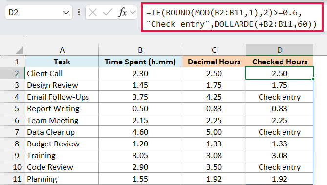
How this formula works:
- The MOD function part, MOD(B2:B11,1), returns the part after the decimal point, such as 0.75 for 3.75.
- The ROUND function rounds that to two decimal places. This matters because Excel stores some decimals with tiny errors, and for larger numbers like 64.60, the MOD function returns a value just under 0.6.
- If the result is 0.6 or more, the minutes are 60 or more, so the IF function returns “Check entry”.
- For every other entry, it returns DOLLARDE(+B2:B11,60), the same result as column C.
Now 3.75, 4.60, and 2.90 all show Check entry, and the other tasks keep their decimal hours.
If you are using Excel 2019 or earlier, enter the below formula in cell D2 and then copy it down to D11:
=IF(ROUND(MOD(B2,1),2)>=0.6,"Check entry",DOLLARDE(B2,60))
In this tutorial, I showed you how to use the DOLLARDE function to convert fractional prices, hours and minutes, and feet and inches into decimal numbers. I also covered the plus-sign trick and how to flag entries with 60 or more minutes.
If you need to go the other way, from a decimal back to fractional notation, Excel has the DOLLARFR function. For example, =DOLLARFR(7.75,60) returns 7.45.
I hope you found this tutorial helpful.
Other Excel Articles You May Also Like:
