

The SYD function in Excel calculates sum-of-years’ digits depreciation. It’s an accelerated method, which means an asset loses more of its value in the early years and less as it gets older.
You give it the cost, the salvage value, the useful life, and the year you’re interested in, and it returns the depreciation for that one year.
This suits assets that lose value quickly when they’re new, like vehicles, computers, and kitchen equipment. Below, I’ll show you how SYD works for a single year, a full schedule, a list of assets, and an asset bought partway through the year.
Follow along with the example file
SYD Function Examples.xlsx
SYD Function Syntax
Here is the syntax of the SYD function:
=SYD(cost,salvage,life,per)
- cost – the price you paid for the asset.
- salvage – what you expect the asset to be worth at the end of its useful life. Use 0 if you expect it to be worth nothing.
- life – the number of periods over which the asset is depreciated (its useful life).
- per – the period you want the depreciation for, such as 1 for the first year or 3 for the third year.
All four arguments are required. The per argument has to use the same unit as life, so if the life is in years, per is a year number.
The per argument also has to be between 1 and the life. Ask for year 6 of a 5-year asset, and SYD returns the #NUM! error because that year doesn’t exist in the asset’s life.
You also get #NUM! when the life is 0 or the salvage value is negative. And if the salvage value is higher than the cost, SYD returns a negative number, which is usually a sign of a typo in the inputs.
The SYD function works in Excel 365, 2024, 2021, 2019, 2016, and Excel for Mac.
When to Use the SYD Function
Use this function when you need to:
- Get the depreciation for one specific year of an asset’s life
- Build a depreciation schedule where the early years carry more of the cost
- Work out this year’s depreciation for every asset in a list
- Compare accelerated depreciation with straight-line depreciation
- Depreciate an asset that was bought partway through your fiscal year
Let me show you a few practical examples of how to use the SYD function.
Example 1: Calculate First-Year Depreciation With SYD
Let’s start with a simple example.
Below are the details of a pizza oven a restaurant bought, and I want to get its depreciation for year 1 in cell B7.
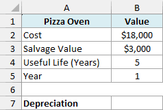
Here is the formula:
=SYD(B2,B3,B4,B5)
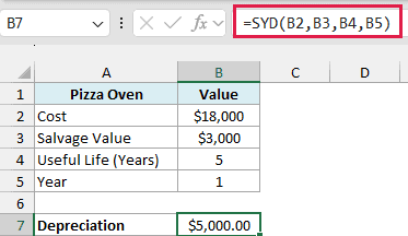
The formula returns $5,000.00, which is how much the oven loses in value in its first year.
Here’s how SYD gets there. The oven has a 5-year life, so SYD adds up the year numbers 5 + 4 + 3 + 2 + 1, which gives 15.
The cost minus the salvage value ($18,000 – $3,000 = $15,000) is the total the oven can lose over its life, called the depreciable amount. In year 1, the oven gets 5/15 of that, which is $5,000.
The top number is the years of life left, counting the current year. So year 2 gets 4/15, year 3 gets 3/15, and the depreciation goes down every year.
Change the year in B5 to 2, and the formula returns $4,000.00.
Example 2: Create a Sum-of-Years’ Digits Depreciation Schedule
Most of the time, you want the depreciation for every year of the asset’s life, not just one.
Below are the details of a box truck a moving company bought, along with the year numbers of its 8-year life, and I want to get the depreciation for each year in column E.
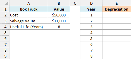
Here is the formula:
=SYD(B2,B3,B4,D2:D9)
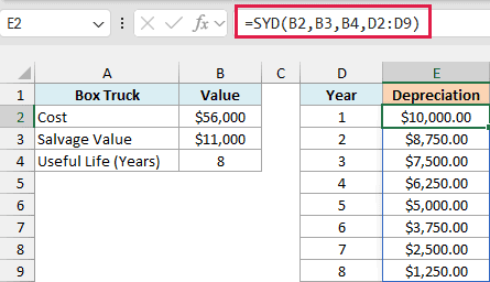
You enter this one formula in cell E2, and it spills the depreciation for all eight years down to E9.
Since the per argument is the range D2:D9, SYD calculates the depreciation once for each year number. The truck loses $10,000.00 in year 1 and only $1,250.00 in year 8.
If you add up all eight years, you get $45,000, which is exactly the cost minus the salvage value. So at the end of its life, the truck is on the books at its $11,000 salvage value.
The cells below E2 need to be empty for the results to spill. If something is in the way, you’ll see a #SPILL! error instead.
Pro Tip: If you don’t have a column of year numbers, the SEQUENCE function can create them inside the formula. =SYD(B2,B3,B4,SEQUENCE(B4)) returns the same eight values.
If you are using Excel 2019 or earlier, enter the below formula in cell E2 and then copy it down the range:
=SYD($B$2,$B$3,$B$4,D2)
Example 3: Get This Year’s Depreciation for a List of Assets
In a real business, each asset is at a different point in its life. A shuttle bus in its fourth year and a TV bought this year don’t get the same share of their cost.
Below is a list of assets a hotel owns, with the year of its life each asset is in during 2026, and I want to get each asset’s 2026 depreciation in column F.
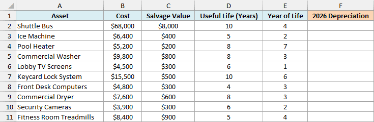
Here is the formula:
=SYD(B2:B11,C2:C11,D2:D11,E2:E11)
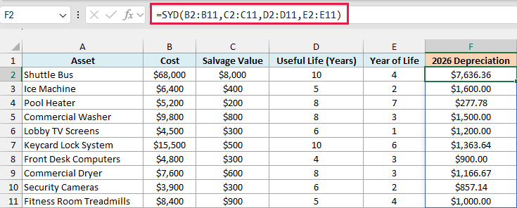
All four arguments are ranges here, so SYD works through the list row by row. It uses the cost, salvage value, life, and year of life from the same row, and spills one result for each asset.
For example, the shuttle bus is in year 4 of its 10-year life, so it has 7 years of life left, counting this one (10 – 4 + 1).
The year numbers 1 to 10 add up to 55, so the bus gets 7/55 of its $60,000 depreciable amount ($68,000 – $8,000), which is $7,636.36.
If you are using Excel 2019 or earlier, enter the below formula in cell F2 and then copy it down the range:
=SYD(B2,C2,D2,E2)
Example 4: Avoid the #NUM! Error for Fully Depreciated Assets
Most asset lists don’t have a “year of life” column. They have the purchase year, and some of the older items have already used up their useful life.
Below is an equipment list from a dental clinic with the year each item was bought, and I want to get this year’s depreciation for each item in column F, using the current year in H2.
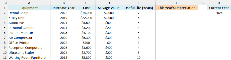
Here is the formula:
=LET(yr,H2-B2:B11+1,IF(yr>E2:E11,0,SYD(C2:C11,D2:D11,E2:E11,yr)))
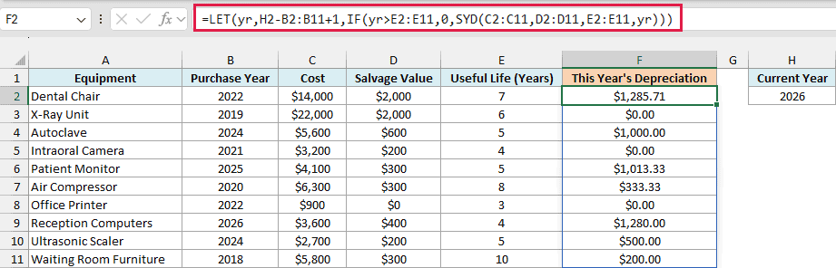
How this formula works:
- H2-B2:B11+1 works out which year of its life each item is in. The purchase year itself counts as year 1, so the dental chair bought in 2022 is in year 2026 – 2022 + 1 = 5.
- yr is the name the LET function gives to that result, so the formula can use it twice without calculating it twice.
- SYD(C2:C11,D2:D11,E2:E11,yr) gets the depreciation for that year of each item’s life.
- IF(yr>E2:E11,0,…) returns 0 for any item whose year is past its useful life, and the SYD result for everything else.
Without the IF check, the X-ray unit, the intraoral camera, and the office printer would show #NUM!. The X-ray unit, for example, is in year 8 of a 6-year life, and SYD can’t return depreciation for a year after the life ends.
A 0 is the right answer for these items, because they’re already fully depreciated. You could wrap SYD in the IFERROR function instead, but that would also hide real mistakes, like text typed in the Cost column, so checking the year is the safer choice.
Next year, change H2 to 2027 and the whole column updates.
If you are using Excel 2019 or earlier, enter the below formula in cell F2 and then copy it down the range:
=IF($H$2-B2+1>E2,0,SYD(C2,D2,E2,$H$2-B2+1))
Example 5: SYD vs Straight-Line Depreciation
To see what makes SYD different, it helps to put it next to straight-line depreciation, which spreads the cost evenly over the asset’s life.
Below are the details of an electric forklift with a 5-year life, and I want to compare its SYD depreciation in column E with its straight-line depreciation in column F.
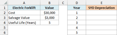
Here is the SYD formula:
=SYD(B2,B3,B4,D2:D6)
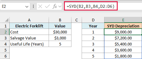
This spills the SYD depreciation for all five years. It starts at $9,000.00 in year 1 and drops by $1,800.00 every year.
And here is the straight-line formula, entered in F2 and copied down to F6:
=SLN($B$2,$B$3,$B$4)
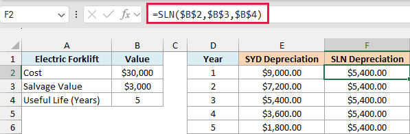
The SLN function returns $5,400.00 for every year, because it splits the $27,000 depreciable amount evenly over 5 years.
Both columns add up to $27,000, so the total depreciation is the same and only the timing changes.
SYD books $3,600 more than straight-line in year 1 and $1,800 more in year 2. The two match in year 3, and SYD makes up the difference with smaller amounts in years 4 and 5.
If you want an even bigger write-off in the first years, the DDB function uses the double-declining balance method instead.
Example 6: SYD Depreciation for an Asset Bought Mid-Year
SYD assumes each period is a full year of the asset’s life. But when you buy an asset in September and your fiscal year ends in December, its first year of life is split across two fiscal years.
Below are the details of a coffee roaster that was in use for 4 months of fiscal year 1, and I want to get its depreciation for each fiscal year in column E.
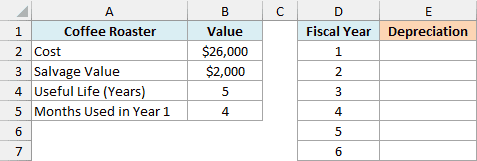
Here is the formula:
=LET(f,B5/12,k,D2:D7,IF(k<=B4,f*SYD(B2,B3,B4,k),0)+IF(k>1,(1-f)*SYD(B2,B3,B4,k-1),0))
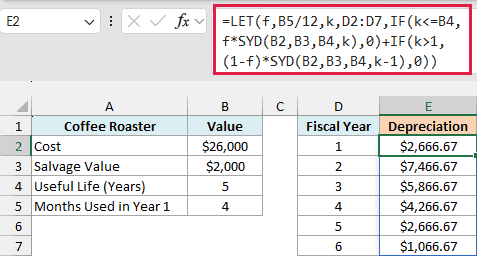
The roaster’s first year of life runs from September to August. So 4 months of it fall in fiscal year 1, and the other 8 months fall in fiscal year 2.
That pattern repeats every year. Each fiscal year gets 4/12 of the current year of life and 8/12 of the previous year of life, which is why a 5-year asset now spreads over six fiscal years.
How this formula works:
- f,B5/12 stores the share of fiscal year 1 the roaster was in use, which is 4/12.
- k,D2:D7 stores the fiscal year numbers 1 to 6.
- IF(k<=B4,f*SYD(B2,B3,B4,k),0) takes 4/12 of year k of the roaster’s life. Fiscal year 6 has no year 6 of life, so this part is 0 there.
- IF(k>1,(1-f)*SYD(B2,B3,B4,k-1),0) takes the other 8/12 from the previous year of life. Fiscal year 1 has no previous year, so this part is 0 there.
For example, fiscal year 2 gets 8/12 of the $8,000 from year 1 of life plus 4/12 of the $6,400 from year 2, which is $7,466.67. All six fiscal years add up to $24,000, the cost minus the salvage value.
The IF checks are needed because SYD returns #NUM! for period 0 and for a period after the life ends. Without them, fiscal year 1 and fiscal year 6 would show #NUM!, and the checks turn those parts into 0.
Important: This formula counts the purchase month as a full month and assumes a 12-month fiscal year. Companies and tax rules handle partial years differently, so check the rule you need to follow before using it.
If you are using Excel 2019 or earlier, enter the below formula in cell E2 and then copy it down the range:
=IF(D2<=$B$4,$B$5/12*SYD($B$2,$B$3,$B$4,D2),0)+IF(D2>1,(1-$B$5/12)*SYD($B$2,$B$3,$B$4,D2-1),0)
So these are six practical ways to use the SYD function in Excel.
It gives you the depreciation for a single year, a full schedule, or a whole list of assets, and with a little help from the IF function, it handles fully depreciated assets and mid-year purchases too.
If an asset loses value at a steady pace instead, straight-line depreciation with the SLN function is the simpler choice.
I hope you found this Excel tutorial useful.
Other Excel Articles You May Also Like:
