

A histogram is a common data analysis tool in the business world. It’s a column chart that shows the frequency of the occurrence of a variable in the specified range.
According to Investopedia, a Histogram is a graphical representation, similar to a bar chart in structure, that organizes a group of data points into user-specified ranges. The histogram condenses a data series into an easily interpreted visual by taking many data points and grouping them into logical ranges or bins.
A simple example of a histogram is the distribution of marks scored in a subject. You can easily create a histogram and see how many students scored less than 35, how many were between 35-50, how many between 50-60 and so on.
There are different ways you can create a histogram in Excel:
- If you’re using Excel 2016 or a later version (including Microsoft 365), there is an in-built histogram chart option that you can use.
- If you’re using Excel 2013, 2010 or prior versions (and even in the newer versions), you can create a histogram using the Data Analysis ToolPak or by using the FREQUENCY function (covered later in this tutorial).
I’ll also show you how to change the bins in the in-built histogram chart, so you get the ranges you actually want. Let’s see how to make a Histogram in Excel.
Follow along with the example file
Histogram in Excel.xlsx
Creating a Histogram Using the Built-In Histogram Chart
Excel 2016 got a new addition in the charts section where a histogram chart was added as an inbuilt chart. It takes just a few clicks, and the chart updates on its own when you change the data.
The built-in Histogram chart works in Excel 2016 and later on Windows (including Microsoft 365) and in Excel for Mac with Microsoft 365. In case you’re using Excel 2013 or prior versions, check out the sections on the Data Analysis ToolPak and the FREQUENCY function.
Below I have the marks (out of 100) of 40 students in a subject, and I want a histogram that shows how many students fall in each range of marks.
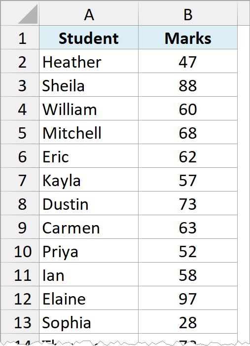
Here are the steps to create a Histogram chart in Excel:
- Select the marks in B1:B41, including the header.
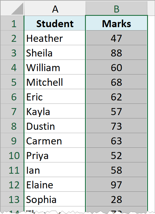
You only need to select the column with the numbers. The student names don’t go into a histogram, because the chart counts values and doesn’t plot each student separately.
- Click the Insert tab.
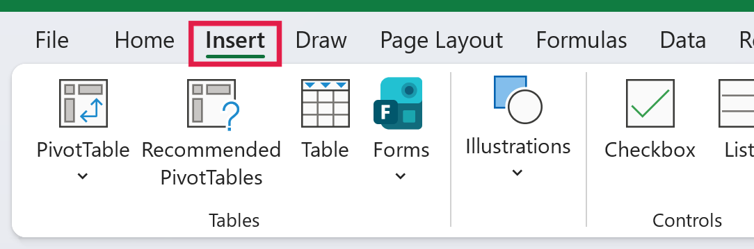
- In the Charts group, click on the Insert Statistic Chart icon.
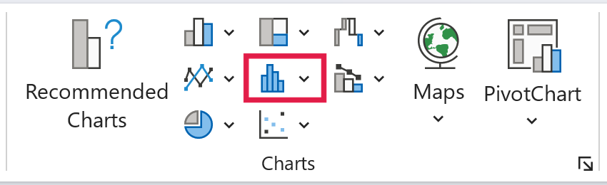
- In the Histogram group, click on the Histogram chart icon.
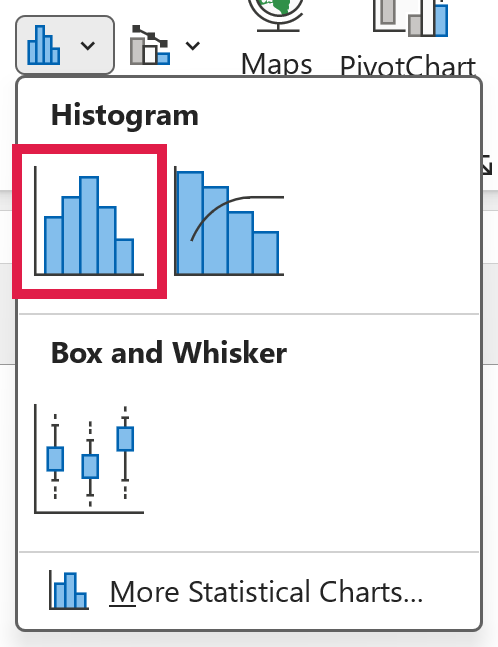
If you’re using Excel for Mac, click the Insert tab, click the Statistical icon, and then click Histogram. You can also get to this chart from Recommended Charts in the Insert tab, under the All Charts tab.
The above steps would insert a histogram chart based on your data set (as shown below). I’ve also changed the chart title to Student Marks.
![Histogram chart titled Student Marks with four automatic bins: [28, 46], (46, 64], (64, 82], (82, 100]](https://trumpexcel.com/wp-content/uploads/2026/11/hist-06-auto-chart.png)
Excel decided on four bins here, and each label below a bar tells you the range of marks in that bin. A square bracket means the number is included, and a round bracket means it isn’t.
So [28, 46] counts the marks from 28 to 46 (both included), and (46, 64] counts the marks above 46 and up to 64. The first bin starts at 28 because that’s the lowest mark in the data.
Since the chart reads the marks straight from the cells, it updates as soon as you change any of them. That’s a big advantage over the Analysis ToolPak method covered later, which gives you a chart that doesn’t update.
How to Change the Bins in an Excel Histogram
Excel picks the bins for you, but you’ll often want different ranges (say, one bar for every 20 marks). You can change them from the Format Axis pane.
Here are the steps to open the bin options:
- Right-click on the horizontal axis (the bin labels below the bars) and select Format Axis.
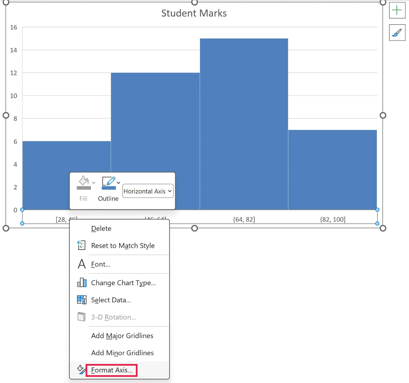
This will open a pane on the right with all the relevant axis options. The bin settings are in the Axis Options section.
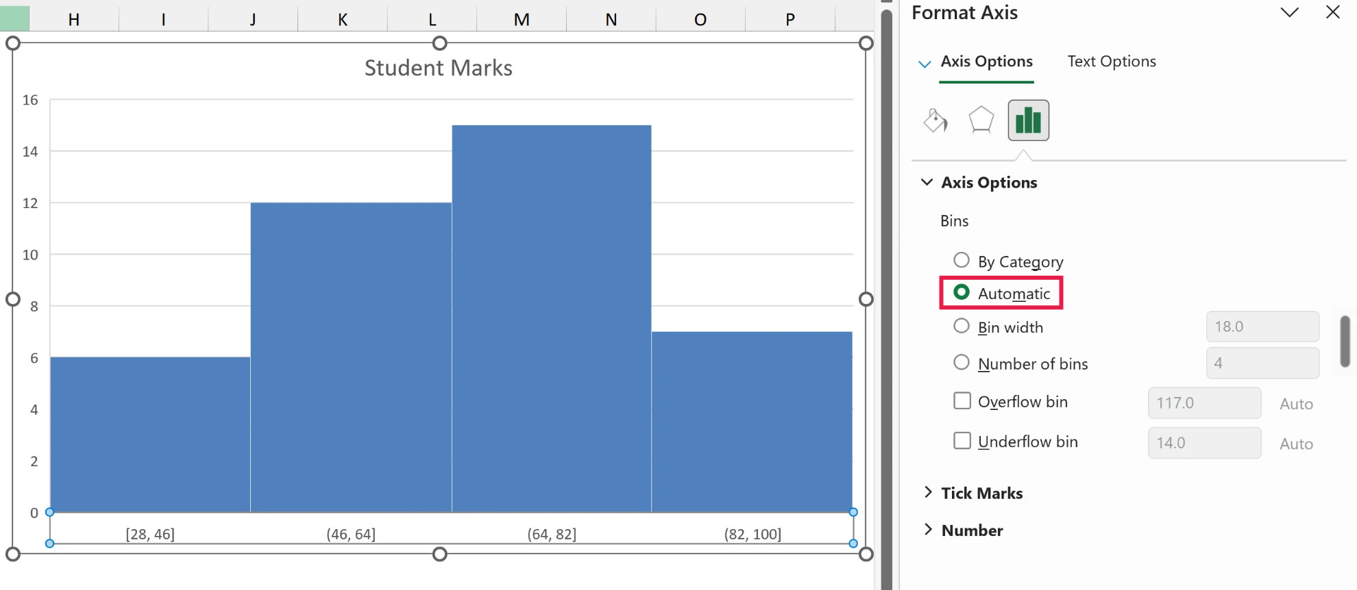
Here are some of the things you can do to customize this histogram chart. Each example starts from the automatic chart, so you can see what that one option changes.
By Category: This option is used when you have text categories. Excel groups the repeated categories together and adds up their values.
For example, if you have sales data for items such as Printer, Laptop, Mouse, and Scanner, and you want to know the total sales of each of these items, you can select both the item column and the sales column and use the By Category option.
It isn’t helpful in our example, as we’ve selected only the marks, so there are no text categories to group.
Automatic: This option automatically decides what bins to create in the Histogram. For example, in our chart, it decided that there should be four bins.
Excel works out the bin width from how spread out your data is (Microsoft calls this Scott’s normal reference rule). You can change it by using the Bin width or Number of bins options covered below.
Bin width: Here you can define how big the bin should be. If I enter 20 here, it will create bins such as [28, 48], (48, 68], (68, 88], and (88, 108].
![Histogram with Bin width 20: bins [28, 48], (48, 68], (68, 88], (88, 108]](https://trumpexcel.com/wp-content/uploads/2026/11/hist-09-bin-width-20.png)
Number of bins: Here you can specify how many bins you want. It will automatically create a chart with that many bins, and if I specify 7 here, it will create a chart as shown below.
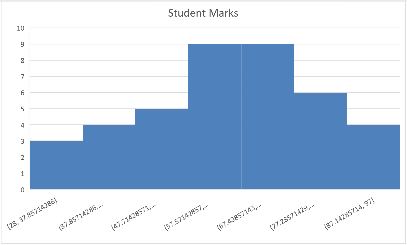
Excel splits the range of marks into seven equal parts, so the bin labels end up as long decimals like 37.85714286. If you want clean round ranges, use Bin width instead.
At a given point, you can either specify Bin width or Number of bins (not both).
Overflow bin: Use this bin if you want all the values above a certain value clubbed together in the Histogram chart.
For example, if I want to know the number of students that have scored more than 75, I can enter 75 as the Overflow bin value.
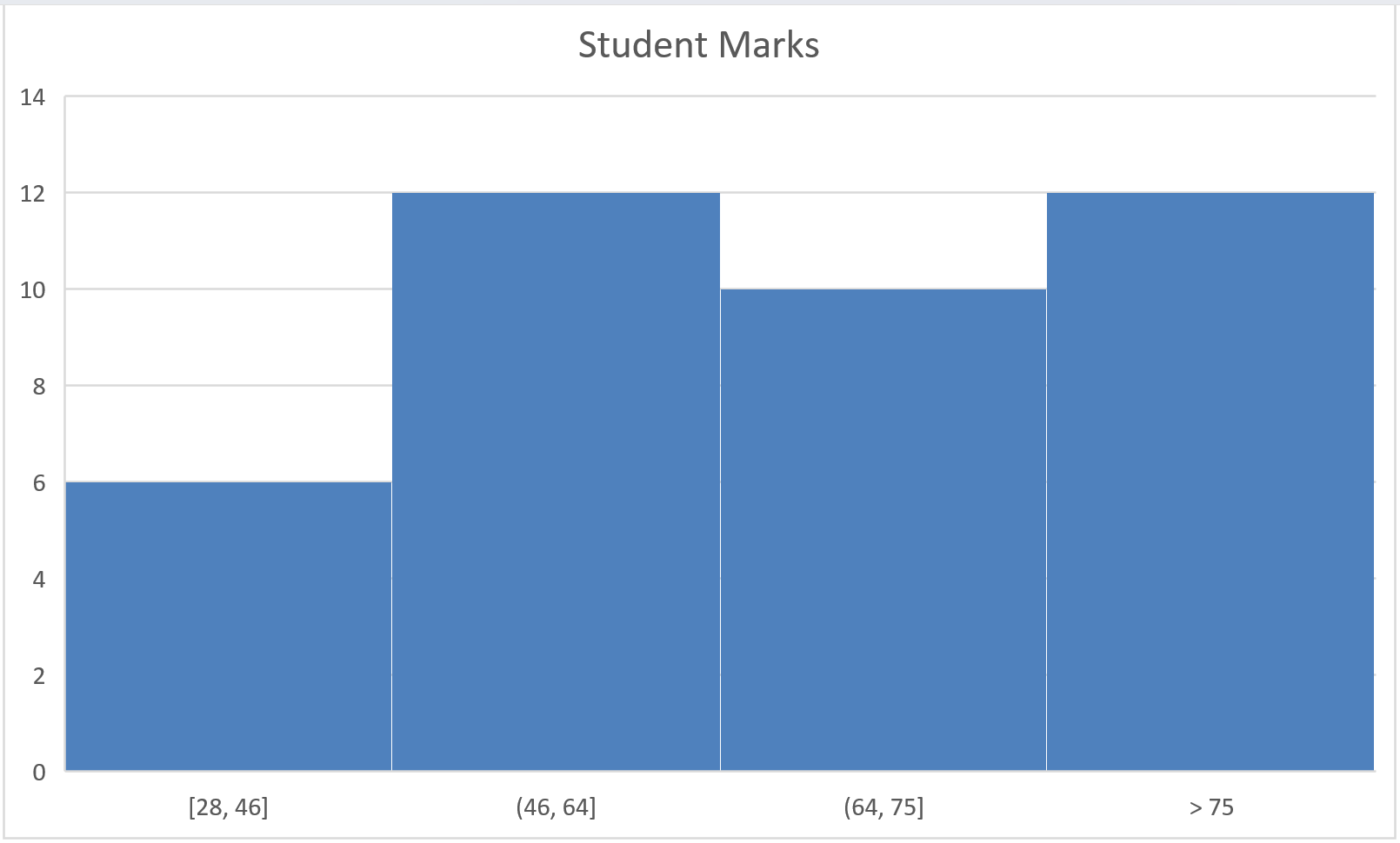
The last bar is now labeled > 75, and it shows that 12 students scored more than 75.
Underflow bin: Similar to Overflow bin, if I want to know the number of students that have scored 40 or less, I can enter 40 as the value and show a chart as shown below.
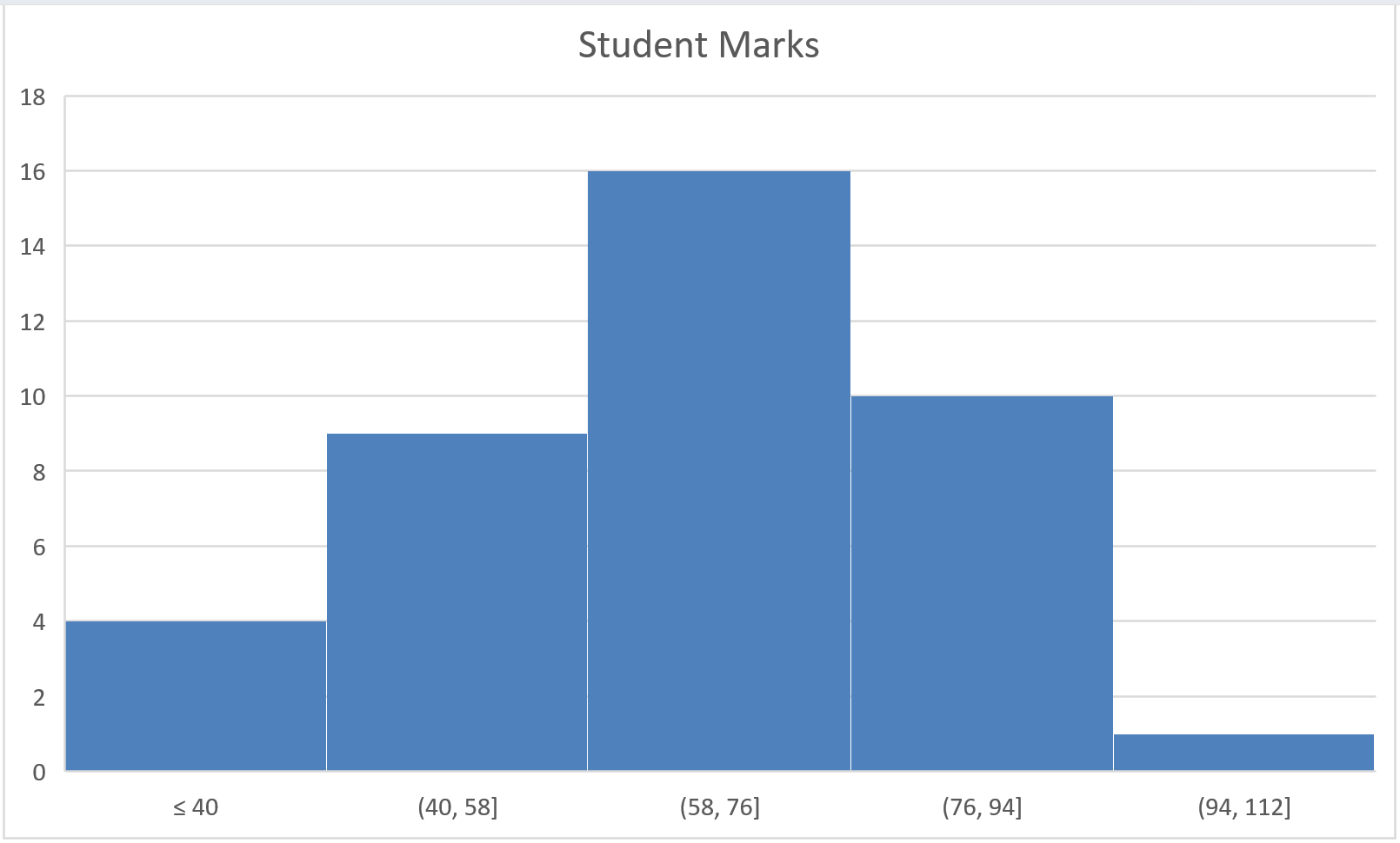
The first bar is now labeled ≤ 40, and it shows that 4 students scored 40 or less. Note that the underflow bin includes the value you enter, while the overflow bin only counts the values above it.
Once you have specified all the settings and have the histogram chart you want, you can further customize it (changing the title, removing gridlines, changing colors, etc.)
Also read: How to Calculate Percentile in Excel
Installing the Data Analysis ToolPak
The Data Analysis ToolPak method will also work for all the versions of Excel (including the newer ones). However, if you’re using Excel 2016 or later, I recommend you use the inbuilt histogram chart (as covered above).
To create a histogram using the Data Analysis ToolPak, you first need to install the Analysis ToolPak add-in. This add-in enables you to quickly create the histogram by taking the data and data range (bins) as inputs.
To install the Data Analysis ToolPak add-in:
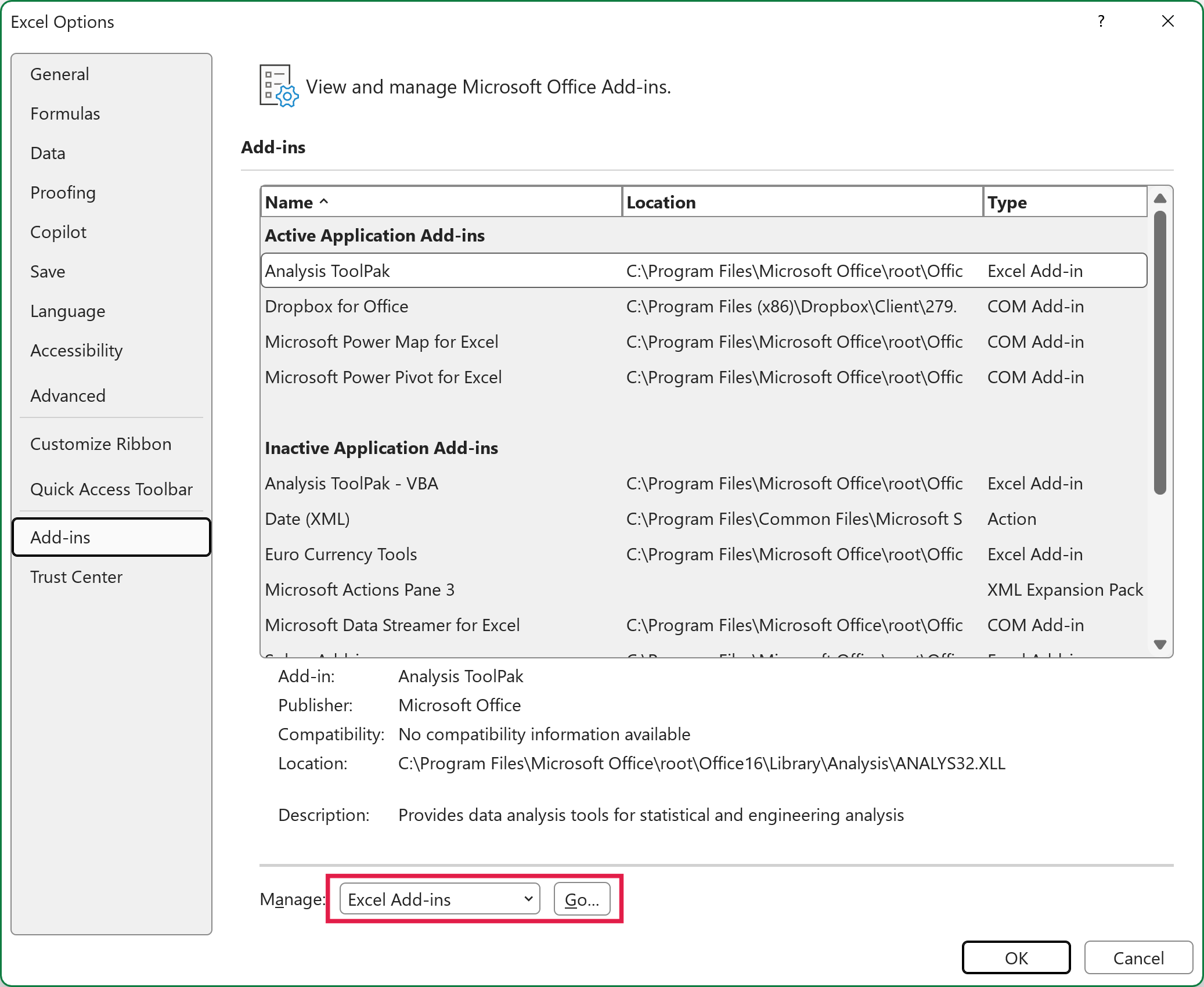
- Click the File tab and then select Options.
- In the Excel Options dialog box, select Add-ins in the navigation pane.
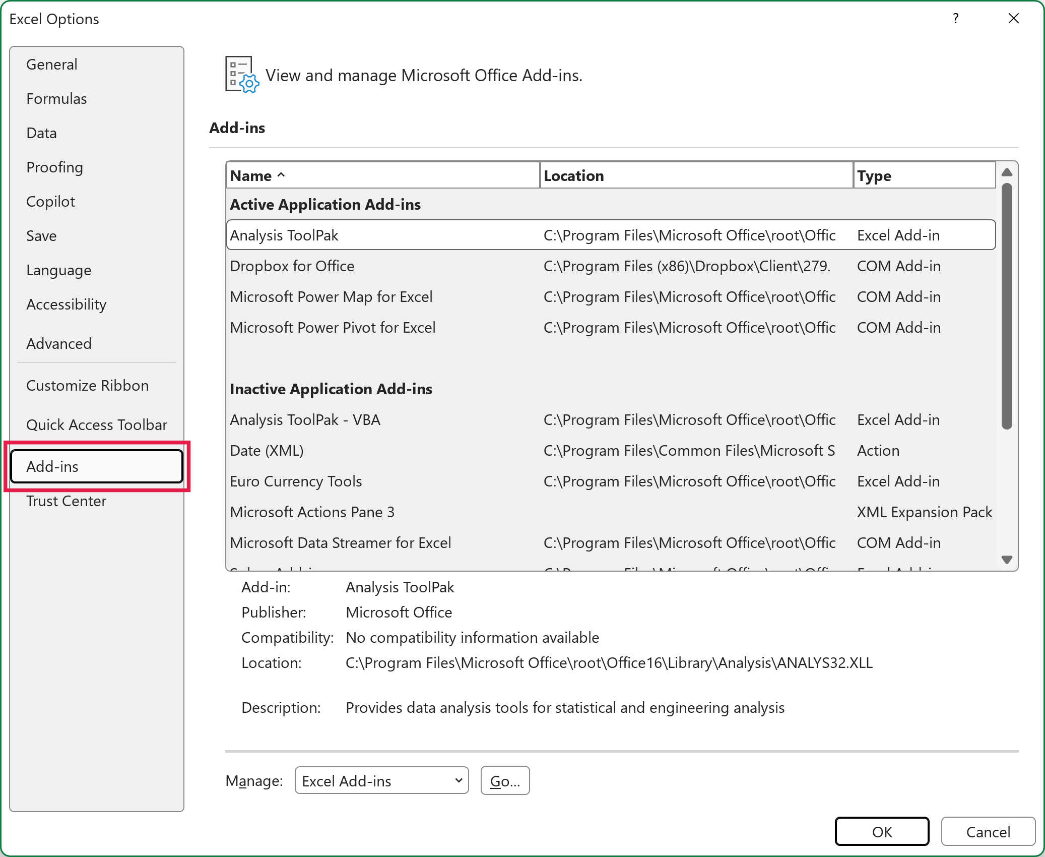
- In the Manage drop-down, select Excel Add-ins and click Go.
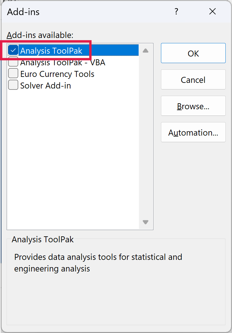
- In the Add-ins dialog box, select Analysis ToolPak and click OK.
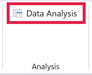
This would install the Analysis ToolPak, and you can access it in the Data tab in the Analysis group.
On a Mac, click the Tools menu, select Excel Add-ins, check Analysis ToolPak, and click OK. Then quit and restart Excel, and you’ll find Data Analysis in the Data tab.
Creating a Histogram Using the Data Analysis ToolPak
Once you have the Analysis ToolPak enabled, you can use it to create a histogram in Excel. If you don’t see Data Analysis in the Data tab, install the add-in first (covered in the section above).
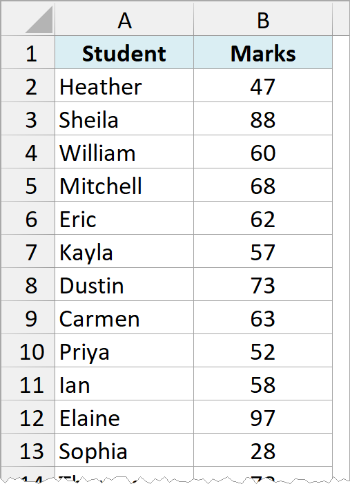
Below I have the same marks (out of 100) of 40 students, and I want the ToolPak to count how many students fall in each range of marks, with the result starting in cell F1.
To create a histogram using this data, we need to create the data intervals in which we want to find the data frequency. These are called bins.
With the above dataset, the bins would be the marks intervals. You need to specify these bins separately in an additional column as shown below:
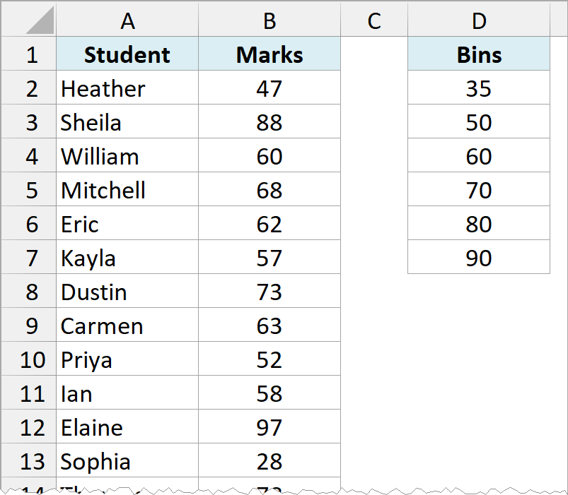
Each bin is the upper limit of its range. So 35 counts the marks up to 35, and 50 counts the marks above 35 and up to 50.
Now that we have all the data in place, let’s see how to create a histogram using this data:
- Click the Data tab.
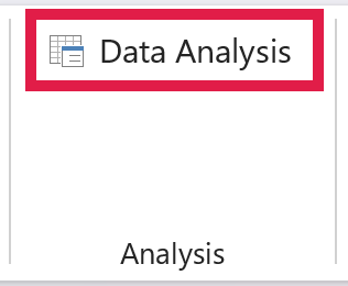
- In the Analysis group, click on Data Analysis.
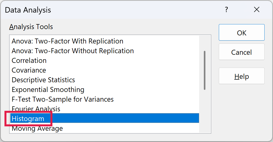
- In the Data Analysis dialog box, select Histogram from the list and click OK.
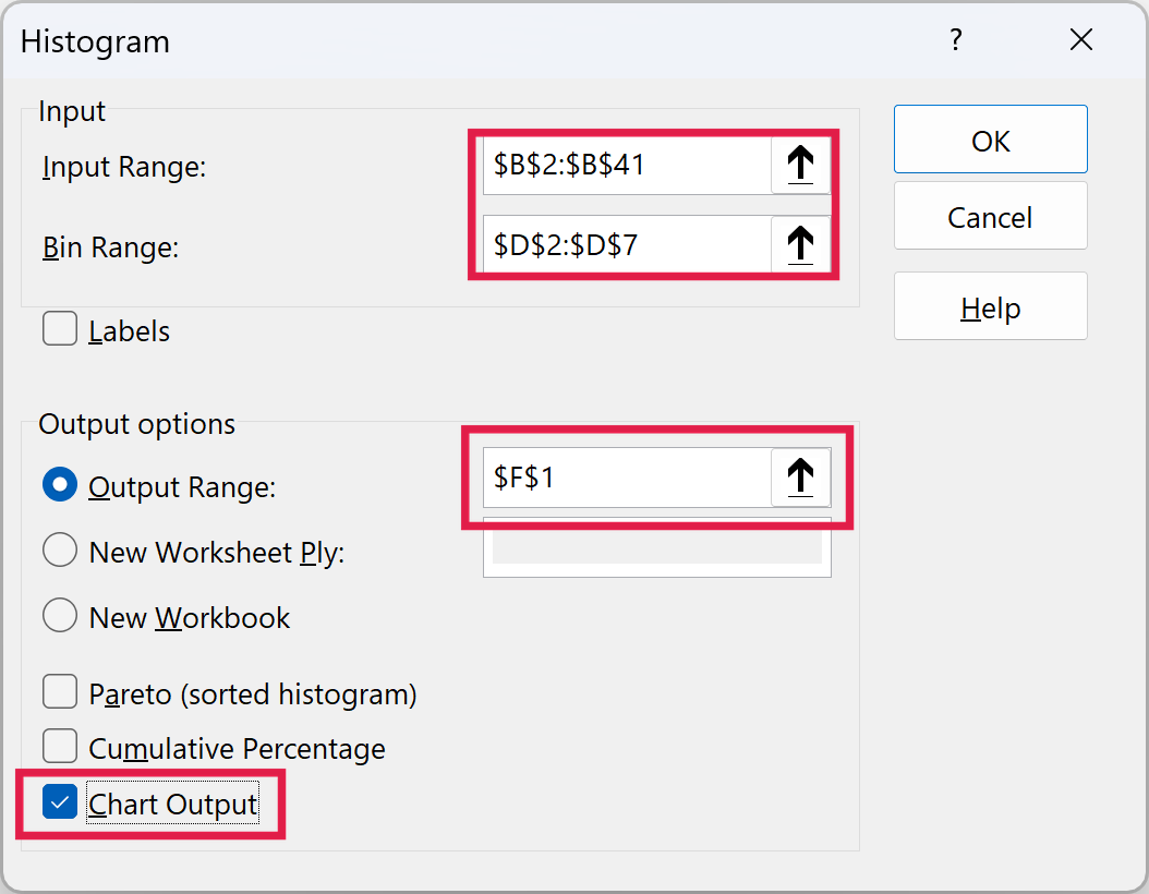
- In the Histogram dialog box, select the Input Range (all the marks in our example, B2:B41).
- Select the Bin Range (cells D2:D7).
- Leave the Labels checkbox unchecked (you need to check it if you included labels in the data selection).
- Select Output Range and specify cell F1 to get the Histogram in the same worksheet. Else, choose the New Worksheet Ply or New Workbook option to get it in a separate worksheet or workbook.
- Select Chart Output.
- Click OK.
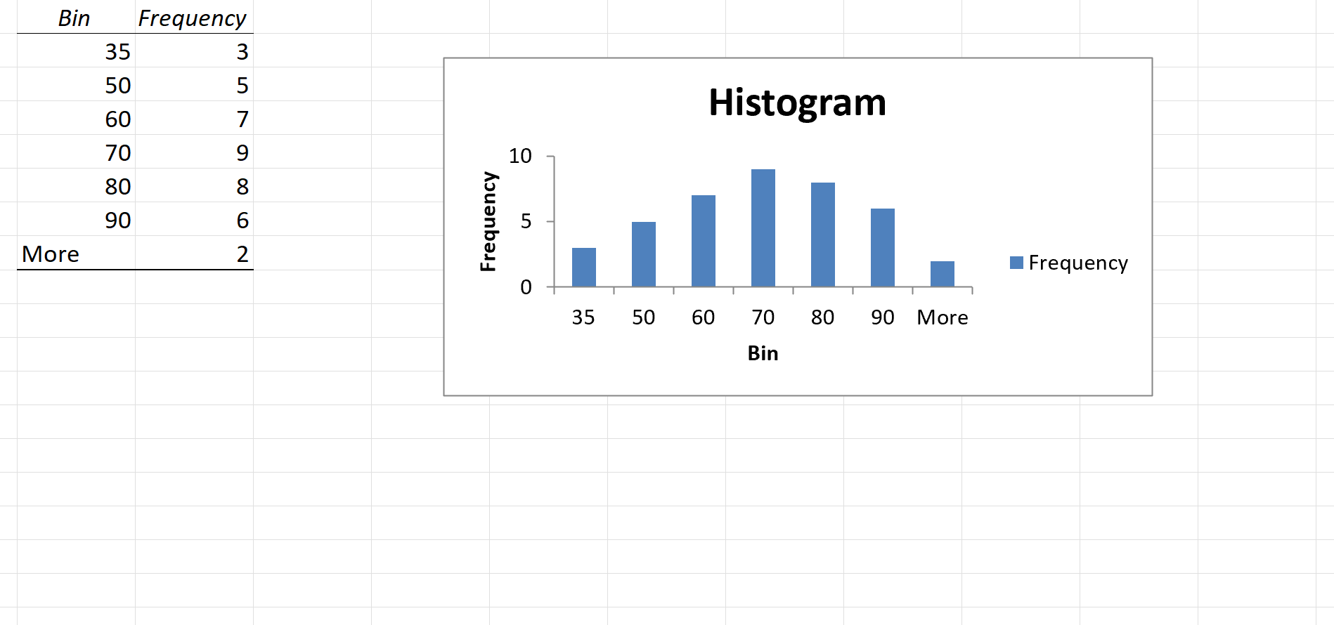
This would insert the frequency distribution table and the chart in the specified location.
Now there are some things you need to know about the histogram created using the Analysis ToolPak:
- The first bin includes all the values at or below it. In this case, 35 shows 3 values, which means three students scored 35 or less.
- In the same way, 50 shows the 5 students who scored more than 35 and up to 50.
- The last specified bin is 90, however, Excel automatically adds another bin, More. This bin would include any data point which lies after the last specified bin. In this example, it means that there are 2 students who have scored more than 90.
- Note that even if I add the last bin as 100, this additional bin would still be created.
- This creates a static histogram chart. Since Excel creates and pastes the frequency distribution as values, the chart would not update when you change the underlying data. To refresh it, you’ll have to create the histogram again.
- The default chart is not always in the best format (for example, it leaves gaps between the bars). You can change the formatting like any other regular chart.
- Once created, you can not use Control + Z to revert it. You’ll have to manually delete the table and the chart.
If you create a histogram without specifying the bins (i.e., you leave the Bin Range empty), it would still create the histogram. Excel automatically creates equally spaced bins between the lowest and highest values in your data and uses them for the histogram.
Creating a Histogram Using the FREQUENCY Function
The built-in histogram chart already updates when your data changes. But if you’re on Excel 2013 or older, or you also want the counts in cells, you need to resort to formulas.
In this section, you’ll learn how to use the FREQUENCY function to create a dynamic histogram in Excel.
Again, taking the student’s marks data, you need to create the data intervals (bins) in which you want to show the frequency.
Below I have the marks with the bins and a label for each range, and I want the number of students in each range in column F.
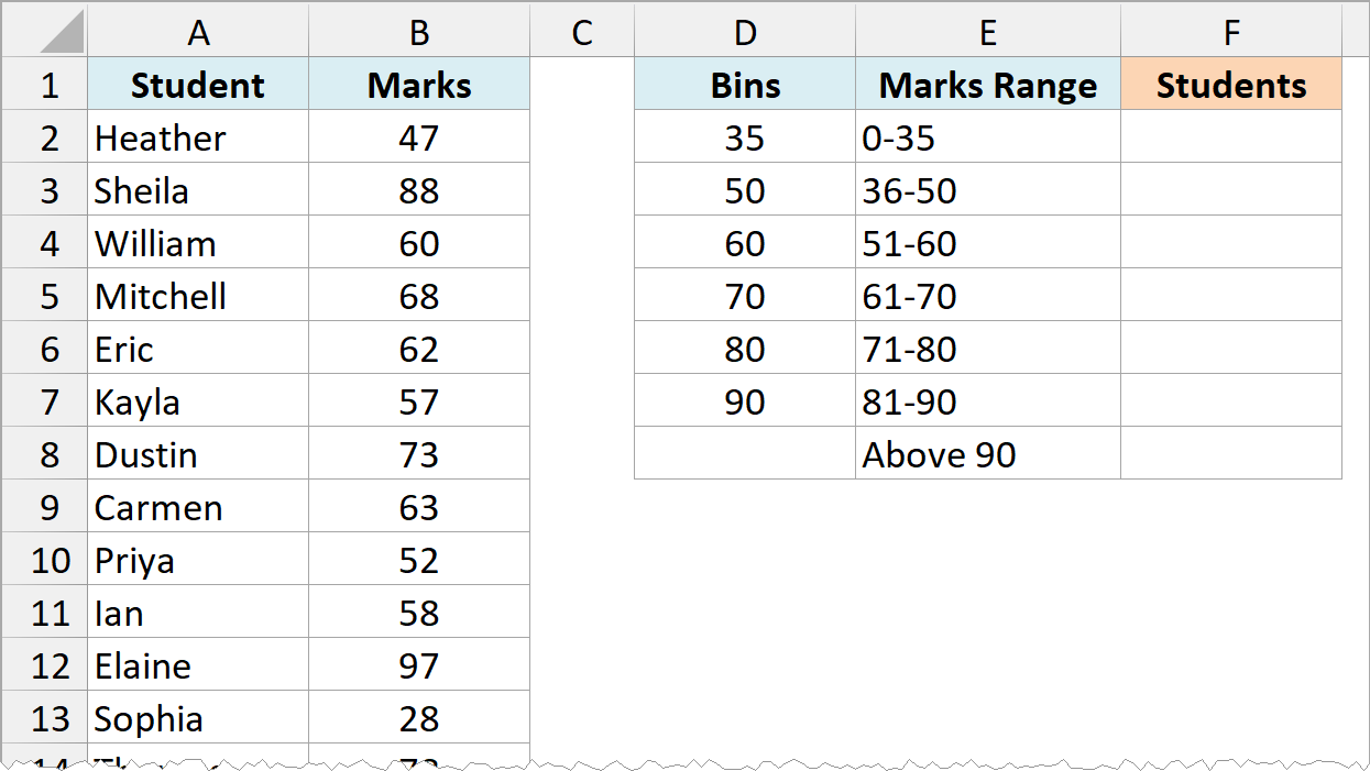
The labels in column E (like 0-35 and 36-50) are typed by hand to make the chart easier to read. The FREQUENCY function doesn’t use them, it only uses the bins in column D.
Here is the function that will calculate the frequency for each interval:
=FREQUENCY(B2:B41,D2:D7)
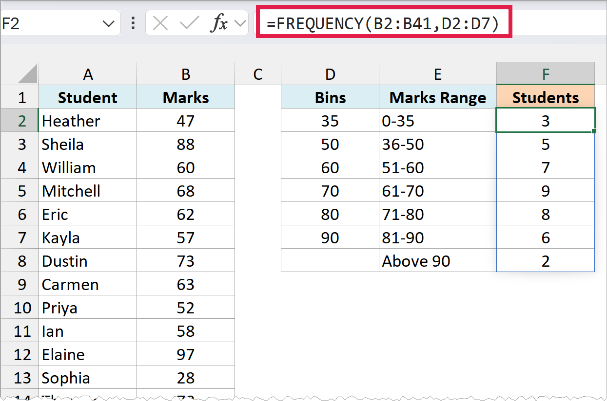
Here, B2:B41 has the marks we want to count, and D2:D7 has the bins they’re counted against.
In Microsoft 365 or Excel 2021 and later, enter this formula in cell F2 and press Enter. The result spills down to F8 on its own, so you don’t need to copy it down or use Control + Shift + Enter.
Notice that there are six bins but seven results. FREQUENCY always returns one more value than the number of bins, and that last value (2 in F8) is the number of students who scored more than 90.
That’s why the Above 90 label in E8 has no bin next to it. If you want all the marks above a value (say, 80) grouped together, just make 80 your last bin, and the extra result will count everything above it.
When a bin is 35, the FREQUENCY function would return a result that includes 35. So 35 means score up to 35, and 50 would mean score more than 35 and up to 50.
The results in F3 to F8 come from the formula in F2, so you can’t edit them on their own. If you type something in any of them, F2 shows a #SPILL! error, and if you need to remove the results, delete the formula in F2.
If you are using Excel 2019 or earlier, select F2:F8 first (one more cell than the number of bins), type the below formula, and then press Control + Shift + Enter:
=FREQUENCY(B2:B41,D2:D7)
In these older versions, the result is an array and you can not delete a part of the array. If you need to, delete all the cells that have the frequency function.
With the result that you get, you can now create a histogram (which is nothing but a simple column chart). Here are the steps:
- Select the labels and the counts in E1:F8.
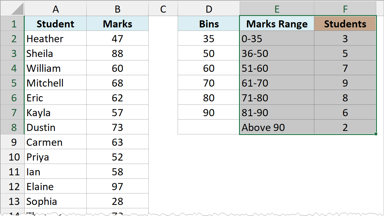
- Click the Insert tab, click the Insert Column or Bar Chart icon in the Charts group, and then click Clustered Column.
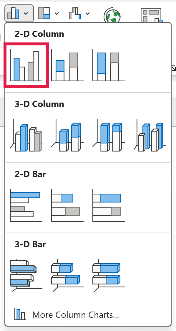
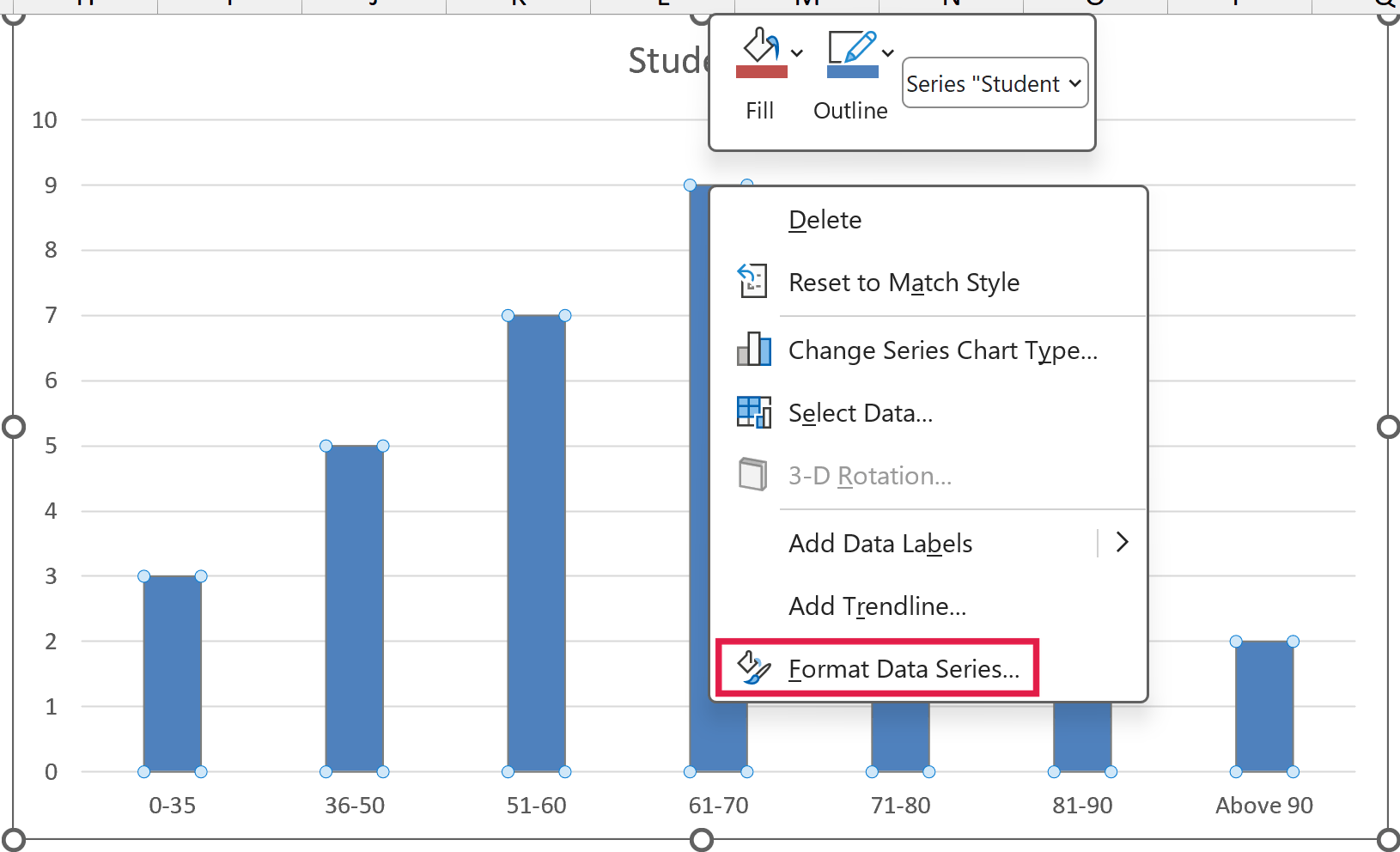
This gives you a column chart with gaps between the bars. In a histogram, the bars touch each other, because each range of marks starts right where the previous one ends.
- Right-click any of the bars and select Format Data Series.
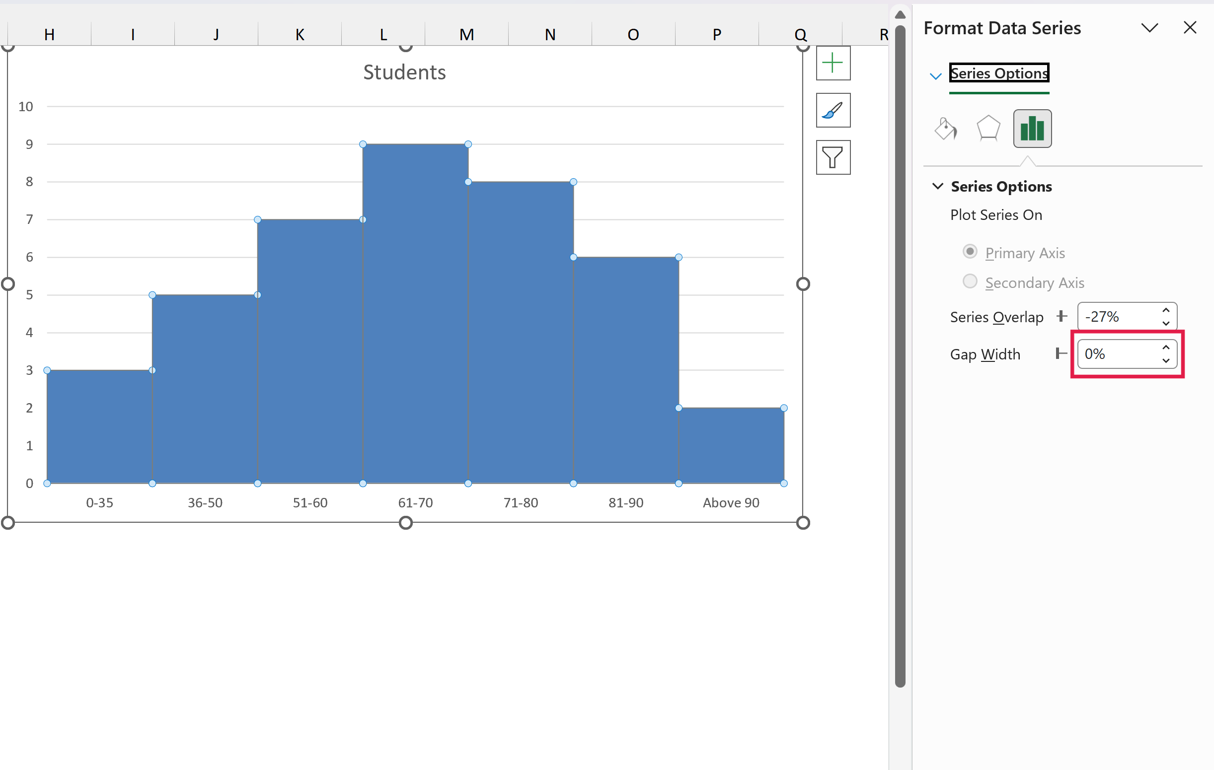
- In the Series Options, change the Gap Width to 0%.
- Click the Fill & Line icon, and under Border, select Solid line and pick white as the color.
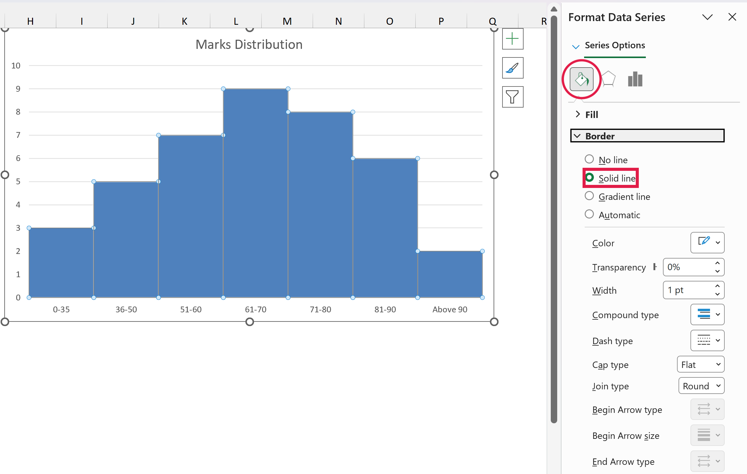
The white border keeps the bars from blending into one block, so each range is still easy to see. I’ve also changed the chart title to Marks Distribution.
Since the counts come from the FREQUENCY function, the chart updates as soon as you change any of the marks.
So these are three ways you can make a histogram in Excel, using the built-in Histogram chart, the Data Analysis ToolPak, or the FREQUENCY function. I also showed you how to change the bins in the built-in chart.
I hope you found this tutorial useful.
You May Also Like the Following Excel Tutorials:
- Creating a Pareto Chart in Excel
- Creating a Gantt Chart in Excel
- Creating a Milestone Chart in Excel
- How to Make a Bell Curve in Excel
- How to Create a Bullet Chart in Excel
- How to Create a Heat Map in Excel
- Standard Deviation in Excel
- Area Chart in Excel
- Advanced Excel Charts
- Creating Excel Dashboards
- How to Group Numbers in Pivot Table in Excel
- How to Get Descriptive Statistics in Excel

WTF??? Trump wouldn’t know what a histogram was if you rammed it up his brain dead ass.
He has no idea how to use excel. What’s up with this moronic website?
Actually your guide line for bar diagram not histogram
Because histogram always for a continuous series in statistics
0-10, 10- 20, 20-30, 30-40, 40-50 and their respective frequencies are 20,30,70,50,and 30
That’s way how draw a histogram?
Please suggest
I use excel 10
This is very helpful tips for data handling
FREQUENCY method doesn’t work, when i hit CONTROL+SHIFT+ENTER the result was number (1) only i don’t know why
Great tutorial it helped heartily
Great post. A helpful tip, if an array needs modifying (i.e., complete the equation or include or exclude cells) press the F2 key while the array is selected and the cursor is in the first cell. This will cancel the CTR+SHIFT+ENTER command and will allow to modify the array instead of deleting it.
Hi Sumit,
When we create histogram using overflow and underflow bin, for overlow it’s showing “>”, and underflow showing “=” and underflow is “<"? I've tried the other option, but didn't find it.
Thank you…
Hello MF,
Yes, creating histogram is easy using the Excel’s pivot table feature. But frankly speaking, if you want to see all the descriptive statistics summary at one go, you should use Excel’s Analysis ToolPak.
Regards
Kawser
Founder http://www.exceldemy.com/
Hi Sumit,
It’s a nice post. Hats off!
Frequency distribution tables have important roles in the lives of data analysts.
Below are my three blog posts on creating frequency distribution tables and its interpretation. In most cases, analysts finish their journey just creating a histogram, but without knowing its four pattern, it is not possible to get hidden gem from the data that makes the histogram. Even I created an Excel template to create histogram automatically.
1) http://www.exceldemy.com/frequency-distribution-excel-make-table-and-graph/
2) http://www.exceldemy.com/how-to-make-a-histogram-in-excel-using-analysis-toolpak/
3) http://www.exceldemy.com/stock-return-analysis-using-histograms-and-skewness-of-histograms/
And my this blog post on statistical data analysis is a must read for the data analysts.
1)http://www.exceldemy.com/learn-today-some-common-statistical-terms-for-data-analysis/
Best regards
Kawser
Founder http://www.exceldemy.com/