

We all use Google as a part of our daily routine. One of its features is search suggestion, where Google acts smart and gives us a list of suggestions while we are typing.

In this tutorial, you’ll learn how to create a searchable drop-down list in Excel – i.e., a drop-down list that will show the matching items as you type.
Below is a video of this tutorial (in case you prefer watching a video over reading the text).
Searchable Drop Down list in Excel
For the purpose of this tutorial, I am using the data of Top 20 countries by GDP.
The intent is to create an excel drop down list with a search suggestion mechanism, such that it shows a drop down with the matching options as I type in the search bar.
Something as shown below:
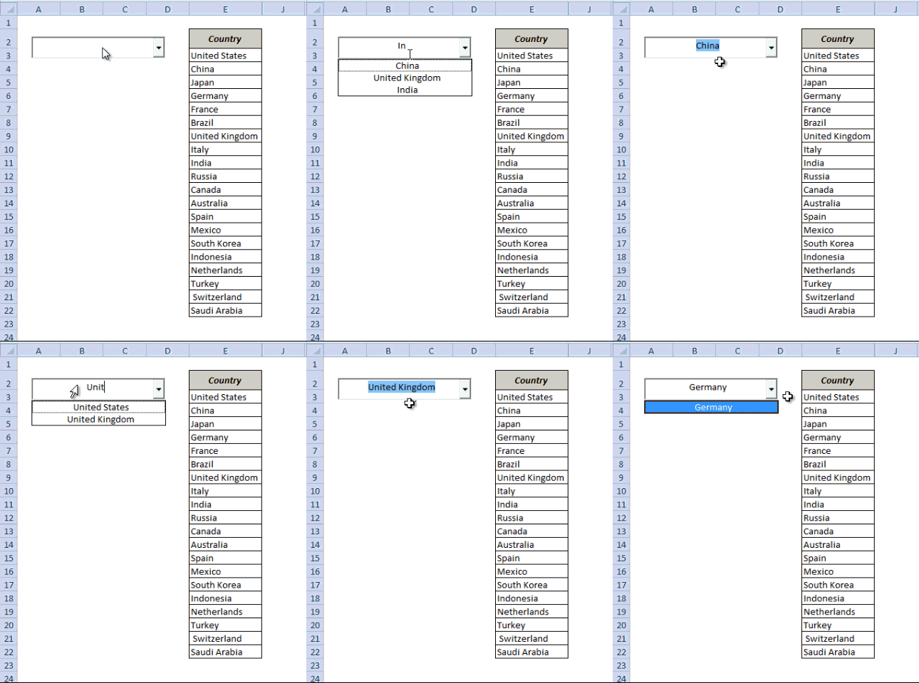
To follow along, download the example file from here

Creating the searchable drop-down list in Excel would be a three-part process:
- Configuring the search box.
- Setting the Data.
- Writing a short VBA Code to make it work.
Step 1 – Configuring the Search Box
In this first step, I will use a combo-box and configure it so that when you type in it, the text is also reflected in a cell in real time.
Here are the steps to do this:
- Go to Developer Tab –> Insert –> ActiveX Controls –> Combo Box (ActiveX Control).
- There is a possibility you may not find the developer tab in the ribbon. By default, it is hidden and needs to be enabled. Click here to know how to get the developer tab in the ribbon in Excel.
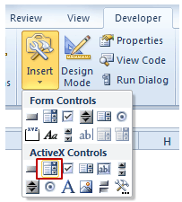
- Move your cursor to the worksheet area and click anywhere. It will insert a combo box.
- Right-click on the Combo Box and select Properties.
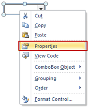
- In the properties dialogue box, make the following changes:
- AutoWordSelect: False
- LinkedCell: B3
- ListFillRange: DropDownList (we will create a named range with this name in step 2)
- MatchEntry: 2 – fmMatchEntryNone
(Cell B3 is linked to the Combo Box, which means that anything you type in the Combo Box is entered in B3)

- Go to Developer tab and click on Design Mode. This will enable you to enter text in the Combo Box. Also, since cell B3 is linked to the combo box, any text that you enter in the combo box would also be reflected in B3 in real-time.
Step 2 – Setting the Data
Now that the search box is all set, we need to get the data in place. The idea is that as soon as you type anything in the search box, it shows only those items that have that text in it.
To do this, we will use
- Three helper columns.
- One dynamic named range.
Helper Column 1
Put the following formula in cell F3 and drag it for the entire column (F3:F22)
=--ISNUMBER(IFERROR(SEARCH($B$3,E3,1),""))
This formula returns 1 when the text in the Combo Box is there in the name of the country on the left. For example, if you type UNI, then only the values for United States and United Kingdom are 1 and all the remaining values are 0.
Helper Column 2
Put the following formula in Cell G3 and drag it for the entire column (G3:G22)
=IF(F3=1,COUNTIF($F$3:F3,1),"")
This formula returns 1 for the first occurrence where Combo Box text matches the country name, 2 for the second occurrence, 3 for the third and so on. For example, if you type UNI, G3 cell will display 1 as it matches United States, and G9 will display 2 as it matches United Kingdom. The rest of the cells will be blank.
Helper Column 3
Put the following formula in cell H3 and drag it for the entire column (H3:H22)
=IFERROR(INDEX($E$3:$E$22,MATCH(ROWS($G$3:G3),$G$3:$G$22,0)),"")
This formula stacks all the matching names together without any blank cells in between them. For example, if you type UNI, this column would show 2 and 9 together, and rest all cell would be blank.
Creating the Dynamic Named Range
Now that the helper columns are in place, we need to create the dynamic named range. This named range will only refer to those values that match the text entered in the combo box. We will use this dynamic named range to show the values in the drop-down box.
Note: In step 1 we entered DropDownList in the ListFillRange option. Now we will create the named range with the same name.
Here are the steps to create it:
- Go to Formulas –> Name Manager.
- In the name-manager dialogue box click New. It will open a New Name dialogue box.
- In the Name Field enter DropDownList
- In the Refers to Field enter the formula: =$H$3:INDEX($H$3:$H$22,MAX($G$3:$G$22),1)
Step 3 – Putting the VBA Code to Work
We are almost there.
The final part is to write a short VBA code. This code makes the drop down dynamic such that it shows the matching items/names as you are typing in the search box.
To add this code to your workbook:
- Right-click on the Worksheet tab and select View Code.
- In the VBA window, Copy and Paste the following code:
Private Sub ComboBox1_Change()
ComboBox1.ListFillRange = "DropDownList"
Me.ComboBox1.DropDown
End Sub
That’s it!!
You are all set with your own Google type Search bar that shows matching items as you type in it.
For a better look and feel, you can cover cell B3 with the Combo Box and hide all the helper columns. You can now show off a little with this amazing Excel trick.
To follow along, download the file from here
What do you think? Would you be able to use this search suggestion drop-down list in your work? Let me know your thoughts by leaving a comment.
If you have enjoyed this tutorial, I am sure you would like the following Excel tutorials too:
- Dynamic Filter – Extract matching data while you type.
- Extract Data based on a Drop Down list selection.
- Creating Dependent Drop Down Lists in Excel.
- The Ultimate Guide to Using Excel VLOOKUP Function.
- How to make multiple selections in a drop-down list in Excel.
- How to Insert and Use a Checkbox in Excel.

Hi there – I have recreated this for a file I use that has 1000 rows. When I search for an entry, say ‘Payroll’ I have about 5 options to choose from. However, my search box just loops my selections like this:
Payroll 1
Payroll 2
Payroll 3
Payroll 4
Payroll 5
Payroll 1
Payroll 2
Payroll 3
Payroll 4
Payroll 5
…And it keeps looping them inside the search box. Any way to get rid of the extra entries so that it just shows the 5?
Hi I wanted to search phone numbers, and everything seems perfect. but problem arrives when the selected comes to the cell it becomes text format. how can I keep it number format please help me
if i want that search drop down list for full row then how is it possible
Hi,
Love your work but i have an issue with the combobox. I can search the data and all works but when i’m continueing entering data in my excel the dropdown keeps randomly appearing even if i selected the data.
is this a bug or did i do something wrong? i have to admit i changed the functions a bit.
since my list was very long where the data is and i add data every day i just added J:J to look for data, not between values.
Can someone help me please?
i think i have the same issue as usman. 4 or 5 posts above. so i use this list to look for names in a client list. what i just noticed is that with some clients the search accepts it and i get a result for my search (the name dissepears in the search field, for other clients the client name stays visible and i constantly get the dropdown… the contactdetails however are filled in so its working correctly
Hey Sumit, thanks again for this awesome tutorial it worked great for me! I am having problems tho when I try to use two on the same sheet. It’s hard to explain but they step on each other, sometimes even causing excel itself to crash. Also when one is selected it shows on the other sheets of the workbook as well. It’s not for work or anything, I just enjoy doing these little projects in excel for my own use. In this case it’s a tool to help me run a gaming server. It’s hard to explain so here’s the file itself… https://www.dropbox.com/s/xnnwyvispzr332b/ARK%20Cheat%20Generator%203.0.xlsm?dl=0
If you could have a quick look it’d be great but I’ll understand if you’re too busy. Thanks in advance!
thank you very much
It took me several attempts to get this correct, but your instructions helped me get through it. Thank you so much!
Hi Sumit,
Thanks for this amazing article – it worked seamlessly when applied to a template I am currently developing. The explanation and code is very easy to follow and implement – so thanks!
I read all the comments, and I’m sure nobody brought this up. I am using the dropdown right now as a reference to pull up entries from a separate datasheet using another activex button. The problem I am encountering is that when the button is clicked, it only runs through part of its code. Currently the logic behind the button is structured as:
If input (cell that dropdown is linked to) is empty, then msgbox “Please select an activity” (action 1)
Else:
If input entry matches an entry in list of activities then call function 1 and function 2 (action 2)
Else msgbox “Cannot find the activity you are looking for” (action 3)
I find that the linkedcell area is always empty once the button is clicked so action 2 never runs. I created another button that just calls function 1 and function 2 (so action 2) and it works, but now the error handling code that I wrote no longer applies (so runtime error every time the cell is empty or if the entry does not match the list).
Any ideas why this happening?
Much thanks!
Amy
I really like your search suggestions in the combo box dropdown list – it is wonderful.
How do I create multiple Combo Box with the same dropdown list within the same worksheet? Using data validation is not good as I have a long list of data.
Hello Megan.. Thanks for commenting.. If you have a huge list, I would suggest you use data validation only. For this technique, you need to create the drop down search bar again and again for each cell.
I have used this formula for a long list of stores i have and it works fine, i tried to just use part of this formula to make it work with my list, i want it to show different columns together as opposed to numbers as you have it here.. for example i have this:
storename | address | phone #
so i used the formula that shows the actual result name, copy pasted into 3 other columns to the left of these, and then i hid the original ones so to only show the resuts after typing in the bar, and i wanted it to give me the results as you see on top so if i have a store i just type the store name and it would show all 3 columns name address and phone #…. but it partially works…. it worked at first when i had 360 rows… then i had to add more stores to the list and then proceeded to modify the formulas accordingly to fit the rows… say i had 380 rows now… i change the formula to row 380 as the end, but then i get an error that it cant work with the formula…. and if i leave it as it was before… it would select more rows than i have… if i have 380 the formula would read like the last row was 760… so it ended up selecting empty rows… if i try to just select the total rows i have it would keep giving me the INCONSISTENT FORMULA error….im confused… all i changed was the total rows in the formula… nothing else … it worked fine before but not now.
what do i do ? what am i missing? please help.
Hi,
The drop down works, but its temperamental. when the drop down appears sometimes it stays there even when i click on another cell. in fact when i enter content in a completely different cell the list from the drop down just appears as though it has a life of its own. any advice on this
Hello Usman.. It seems to working fine on my system. What version of excel are you using?
hi sir, it works but it’s really slow and when i select an item from the list it doesn’t appear immedietly in the box i have to select it and double click it
.
Hello.. Do have a huge data set? I assume it would become slow when you have a huge data set as there are multiple helper columns at play here.
Brilliant this makes my job a lot easier, thank you. I have some problem…I do this and when using it..type to search in that searchable-dropdown and delete it to type new word….and after then I save and all my data in column “H” gone.Thought it causes from deleting..so my question is how can I have searchable drop down with non-editable option.
i created the drop downlist as above.Now how could i extend it to whole column as i want it to each and every cell. I am unable to select the dropdown control box to paste it to remaining columns.
Thank you! Not only for your help with the activeX component, but also your reference below to the VBA method 🙂 That is what I’m going to use! 🙂
Thanks for commenting.. Glad you found it useful 🙂
Hi.
Thank you so much for this tip!
Is there any way to make the link cell dinamic? I want to apply this combobox to work in diferent cells from the same column. Also the list of data is in another worksheet within the same workbook.
WOW! This is ALMOST exactly what I was looking for. Is there a way to have multiple search boxes linked to corresponding cells in the “B” column? I’d like to have the entire B column to be linked to separate search boxes.
Great tutorial Sumit!!! I have only one, even simple question. Each time when I open the worksheet the last entered or chosen value is shown. Is it possible that when opening the worksheet the value is reset (the data in the dropbox should remain intact, only the previous value should not be shown, should be blank)
Thanks in advance
i am not able to write file name “DropDownList” in list fill range whenever i write after clicking file name disappear??? please help
same here, please help
Thank you thank you thank you! This is precisely what I wanted, not to mention perfectly explained!
Thanks for commenting.. Glad you liked it 🙂
Can you do this with multiple cells (say 400) without having to continuously redo every step?
Hello Lexi..This can not be done for a lot of cells at once. It needs to be one by one for all cells. If you want to do this for 400 cells, I suggest you use data validation drop down list
Hi Sumit,
First of all, thanks a lot for this great tutorial and this great idea.
I am now working to implement this, such that the combobox is invoked inside of the cell I am presently in, and it works accordingly. I am relying on the Workbook.SelectionChange event for this. However, I am having some trouble in doing this. I believe it is because the
With
.ListFillRange = DropDownList
.LinkedCell = LinkingCell
End With
is creating some problem. Any suggestions?
Have you already got something like this?
Also, I am working on reducing the 3 lines of helper columns into a small VBA code (using arrays to handle the data), mainly for performance reasons. I will share it with you as I get done.
I want to use a list on a different worksheet. I created the 3 helper cells but in the first one, I tried inserting the worksheet name where the combobox is placed (worksheet named “AGENTS”) with the following formula =–ISNUMBER(IFERROR(SEARCH((AGENTS!$K$2),E3,1),””)) . For some reason the only name it returns is the name on row E11 and it completely fills rows F and G with 1 and row H with the name on row 11. Is it possible to do this with the drop down list being on a separate worksheet?
Hi this works for me, however when I type data into another worksheet the drop down shows up there as if I need to re-select my option. Any help would be greatly appreciated
Change VBA code like this:
Private Sub ComboBox1_GotFocus()
ComboBox1.ListFillRange = “DropDownList”
Me.ComboBox1.DropDown
End Sub
Just copy and paste answer from Sumit Bansal :d
on backspace the content entered and typing again, it wont suggest
easily guided……thanks a lot
Sumit – this is absolutely great, thanks for posting it. I tested the file and it worked fine. But then I tried adapting this for a similar problem, where instead of countries I have a list of about 250 Part IDs (which can be numeric, alpha, or a combination thereof). The issue I have is that Excel seems to crash every time I’m in the Combobox and happen to hit the down arrow key. Maybe it’s something specific with the down arrow key, or maybe 250 rows is “too much” for the formulas? Have you experienced this? Any thoughts?
Thanks for commenting. When I press the down arrow key, it doesn’t crash, but I am also unable to navigate through the list (it just picks up the first matching entry). I tried it with about 500 records and works fine with more data. It seems its the down arrow key creating the trouble
Even same issue in my excel as well.. please help to resolve this.. every time it crashes when I press down arrow.
Thanks a lot. I did it with work sheet but encountered an error that is whenever i search something excel shows same thing in blue color below the combo box or somewhere else on the page. see below screen shot:
Hi did you ever find a solution to this, I’m having the same issue.
Thanks
hi sir how to add more countries or another things? i add more but the combobox is not showing it can u help me sir
Hello, thank you very much for the nice tutorial! It’s really great! I have however an issue. I have Excel 2013, the dropdown works as expected, however when I have the values in my dropdown and I click the ‘down arrow key’ from my keyboard Excel freezes and shuts down. Moreover, this dropdown appears also spontaneously on other sheets(!). Any idea? Moreover, is it possible that this dropdown is integrated as a native dropdown from excel? (maybe using the Data validation?)
Thanks a lot!
We would like to use multiple combo boxes on the same sheet with this approach and have the problem that the comboboxes interfere with each other. Do you have any possible solution here?
Dear, Trumpexcel
can see from the video the created combo box is linked to a cell now my question is can the combo box link to multiple cells in the same column?
Thanks so much in advance
similarly, i need to do it in cell ? please help!!!
Thanks so much for sharing this amazing trick! But i have almost a problem, the combo box shows all the time in another sheets or another excel file…how do I prevent this? I ve read alla the posts before, but the solutions didn’t Work so far…(i meam the vba focus one)…
Thanks in advance
Greetings from italy
First and foremost, Thank You for sharing this information. I have one question that I hope you or someone in this Discussion can answer for me. I used the Drop Down List technique in a form and it worked, but the only thing is that when I tab to my next field in my form, the drop down menu opens the list back up. I provided a screen shoot of what I am talking about. Is there a way to keep the combo box from making the list show the selected data again?
I’m sorry the picture is a bit small but if you can manage to see, the top half shows the selected item in the list and everything is fine. The bottom half shows when I type something else in another field in the same sheet and tab out of that field, the list provides the same selected item in blue again.
Thank You for your assistance!
Nevermind about the picture being small, when I was uploading it, the picture seemed small but when it posted …. whoa, it was huge. Sorry about that you all.
DV
I am facing the same issue, please let me know if you have resolved it. Many thanks
I copy the answer for you :
Private Sub ComboBox1_GotFocus()
ComboBox1.ListFillRange = “=DropDownList”
Me.ComboBox1.DropDown
End Sub
Thank you for sharing this .
However I am getting issue When I use arrow keys (down) to move the selection down the dropdown list to select say 3rd item. Only the first item is selected and dropdown list disappears .
What I want is , when I use arrow keys(up/down) to move the selection up and down the dropdown list, it should only scroll up/down and it should not change the value of the combobox (and fire the change event) until the user hits enter or tab .
Please help.
Hi, one question. How i can do to have the same drop down list with search suggestions in the diferents sheets?
I am trying this since two days, I found difficulty, search suggestion below combo box is not populated, I think I am erring in combo box property set or in macro setting, I put all data according to your video, also downloaded your excel, In your excel file it works, but in my file search suggestion is not showing in drop down list, I think I am missing some thing, can you please guide me in setting, Thanks a lot in advance
how to make a bill using this search box to include those item only which require on respected cells
Hello again,
I’m not very confident with ComboBox so I tried using data validation for a simpler solution.
I used the same helper columns and put my data validation list box below B3 (i.e. B4). The data validation source is =OFFSET($H$3,0,0,MAX($G$3:$G$22),1)
The drawback of this method is that the dropdown list does not change as you type and you type into a different cell from the dropdown (you just enter/press return when you have keyed your search text).
As I say, not as complete or elegant as your method but it means that you don’t need to use Developer or Visual Basic. May be of use for people with large and/or complicated spreadsheets.
HI Joe,
Still at basic Excel level but I have replicated Sumit’s amazing solution exactly – it works wonderfully. I am trying to use your method since I
HI Joe,
Still at basic Excel level but I have replicated Sumit’s amazing solution exactly in a test file – it works wonderfully. I am trying to use your method since I have a worksheet with a long item list, have already created the Validation drop down in another worksheet form – it all works but I would love to be able to search. To try your solution before adding it to my work, I have used your formula as the Data validation source, copied all of Sumit’s formulas and columns skipping the first step of configuring the search box and also no VBA code. However, typing India into cell B3 brings the choice of Turkey in the drop down box, I have tried it several times. Is there something I am missing, would really appreciate your help, I am almost there!
Joe, I tried something ridiculous, changed the cell address of Sumit’s formula in Helper 1, then changed it back to it’s proper address – it suddenly began to work, with your method! Thank you for this solution, and thank you Sumit for this site, even for an absolute beginner like me it is totally amazing!
Hi Lillian,
I’m glad you were able to sort it out.
I’ve added some screenshots for reference showing the data validation source, various cell formulas and the resulting drop down list.
Cheers,
Joe
Thank you Joe. When my workbook was perfect, I tried to Lock/Hide the cells containing formulas and then to Protect the worksheet. Suddenly the drop down list did not work even when I unchecked Hide, Unprotected the sheet, and Re-Saved. Gave up for the day, opened it today and now it works perfectly although I did not change anything at all! Since I had flaky seeming trouble last week, I repaired Office then, hoping that was the issue, but obviously I have a problem – or maybe Excel needs some time to ‘register’ changes:-) Since I am new at excel but with your and Sumit’s help I have done something so way above my level – is this behaviour normal? Also, is there a problem with Protection and Drop Down Validation?
Thanks, Lillian
Hello again Lillian,
Hiding columns will have no effect on how your spreadsheet works. Locking cells and protecting the worksheet is different. By default all cells in the worksheet will be locked when you protect the worksheet so the data validation cell will be locked and therefore will stop working. You can change the default so that all cells are unlocked and then specify just the cells you want to lock. Use Ctrl+Shift+F to get to the Format cells dialog box and use the Protection tab. So highlight the whole worksheet, press Ctrl+Shift+F and unclick the locked cells box in the Protection tab. Then highlight the cells you want locked and click the locked cells box. Then protect your worksheet.
Hope this works ok for you, Joe
Thanks, worked perfectly. Next thing to try, your solution to only result in all records starting with ‘a’. It did work on my sample file which replicates Samit’s tutorial using his version of your solution, but not with my own workbooks. I assume it should work the same way with my list, which is a combination of numbers and also text, but the entire column is formatted as text (I am discovering that this is quite a confusing issue). I will go through your screenshots carefully and hope I can find where I went wrong. Since my source is in another workbook there is ample opportunity for a newbie like me to err with these long formulas…
Thank you so much for doing this, Lillian
Hi, Thanks for sharing this. Can I be so bold as to suggest a possible improvement.
My list is very long so when I type in, for example, “a” I get all the records with an “a” anywhere in them.
What I really wanted was just those records STARTING with “a”.
So I created a new formula in cell J3 which was =LEN(B3).
Then I edited cell F3 to be =–ISNUMBER(IFERROR(SEARCH($B$3,LEFT(E3,$J$3),1),””)) and copied down.
Any thoughts?
Hi Joe.. Thanks for sharing.. And it makes sense when you have a big list. Here is another formula that would work
=–ISNUMBER(MATCH($B$3&”*”,E3,0))
I used it in F3 and copied down.
Hi,
Yes thanks, much more elegant than my attempt.
Cheers
Thanks much for the tip. After getting it to work, I tried to create a second combo box to do the same thing. I created three more helper cells and a new named range, that part works. The trouble is when I am entering data in the second box. I can add data in the firs all works great. When I attempt to add data in the second, the choices in the first re-appear, and nothing appears in the second????
Thank you for posting this topic it was very helpful, but I have a question about how to create multiple cells having that drop down list and giving me the suggestions, is there any way to do it without the box, I would like to have it in the actual cell and for every single cell in the column, Thank you very much
Hi David
did you managed to get answer to your question? if do kindly share with me at danny.tan9090@gmail.com
Hello very good articel. There is one thing you might can help me with. How can i search the data in more then one column? For a better understanding. My data has a title column and a matchcode column. In the title are more detailed informations and in the matchcode its only a single string. But i need to search both of them for the same search string and then combine the results in one named range. Thank you in advance. Greets from Berlin. 🙂
Hi Sumit,
Great job. I’m trying now to adjust it for myself on VBA Form.
Almost everything works….But.
I have combo box on my form and procedure for it. I’m adding to cell B3 what I’m typing.
Private Sub ComboBox1_Change()
Dim vCombo As Variant
vCombo = Me.ComboBox1.Value
Sheet6.Cells(3, 2).Value = vCombo ‘ add combobox value to cell B3
End Sub
Filtered Dynamic DropDownList is appearing, but I can select only FIRST item from list.
If i’m selecting any following items – it’s becoming blank..
Earlier I used the same as yours formulas before. Just without Combo box on sheet.
Instead of that I used formula =CELL(“contents”) in cell B3 (referring to your lesson) – with this you will get value to B3 from any cell in sheet you will type in.
And I have copied Name Validation to all cells I need. It filters list only after I press drop down arrow, but i was enough for me. Now I would like to create that in VBA form.
I’m not professional in Excel, but thinking about possibilities to create that using dynamic arrays and filter them only using VBA code. I need ~30 combo boxes on the form doing the same..
Waiting for you tutorial about it on VBA form..
have you invoice and inventroy software in excel tutorial?
This was incredibly helpful! Thank you very much! My search suggestion seems to be populating options that do not appear in formula, any clues as to why?
Hello Carlos.. Thanks for commenting.. The drop down would show the values in the named range (DropDownList in this example). This would indicate an issue in the formula in named range (=$H$3:INDEX($H$3:$H$22,MAX($G$3:$G$22),1)). Make sure that the reference are absolute (such as $H$3). If this doesn’t work, it would be great if you could share the workbook so that I can have a look
my references are absolute. My formula seems a little different than what you posted but matches what you had in your video. I have COUNTIF instead of MAX… would that be it? How can I share my workbook through here?
You can share your workbook in Dropbox or Onedrive and share the link here
https://www.dropbox.com/s/7uanb2fjj60m2dz/ECC%20PreReqs.xlsm?dl=0
If you enter CIS into any of the search bars you will see what I am talking about (hopefully). Also, I just noticed when I choose CIS 13 it populates CIS 136 (another choice).
Thanks for sharing the file. Everything else works perfectly. The reason CIS 13 entry shows both CIS 13 and CIS 136 as it matches both. But it takes the first matching value, which is CIS 13. Also, use the below code (use change instead of getfocus)
Private Sub ComboBox1_Change()
ComboBox1.ListFillRange = “DropDownList”
Me.ComboBox1.DropDown
End Sub
Sumit, Thank you very much for taking the time to look over my file. I wanted to really express my appreciation for the website that you have built. I cannot thank you enough for taking the time to share your knowledge and expertise. THANK YOU!
PS thank you for your prompt response!
Thank you for your prompt response! My formula looks a little different than yours but I followed your video very closely. My reference is absolute but I am using COUNTIF instead of MAX. This is my formula: =$E$2:INDEX($E$2:$E$410, COUNTIF($E$2:$E$410,”?*”)).
Both formulas are fine. Your formula is correct for the named range. Would be great if you could share the file (a link of the file in dropbox or onedrive)
https://www.dropbox.com/s/7uanb2fjj60m2dz/ECC%20PreReqs.xlsm?dl=0
sorry I think I keep posting twice, it doesn’t seem to register the first time but then it does.
Its when I type CIS that I notice it gives me all those extra options. I also noticed when I choose CIS 13 it populates CIS 136
This is so awesome, thank you! I have a question: (I haven’t checked all my dropdown choices but) One of my drop down choices, once selected, read something else. For example I choose CIS 13 but it shows up as CIS 136 (which is also one of my dropdown choices). The formulas are working correctly and showing all the appropriate choices… I have no clue why it is happening.
Dear Sumit Bansal,
You are great and wonderful working on excel and I want to give you specially thanks and appreciate for your working . I m also teaching advance excel in our local area and I have a question regarding your working “excel drop down list with search…..”
Dear I want to this kind of search engine in one particular column for typing data entry, I want to working on active cell and don’t want combobox, creating search engine on each cell with list (Data validation) or through vba…
Is it possible??
Hope you are understand what I mean to say.. 🙂
Regards,
Mehar Khatri
Hello Mehar.. Thanks for commenting and for your kind words. The above mentioned process can work for a single or a couple of drop downs. For getting it in all active cells, VBA would be the way to go. I will soon write the code for it and share with you. It is definitely on my To Do list now 🙂
This is brilliant!
Thanks for the comment. Glad you liked it 🙂
Thanks for commenting.. Glad you liked it 🙂
Hi Sumit!
Good job! Just one remark. I found that this option works much better.
Got focus -> Change
Private Sub ComboBox1_Change()
ComboBox1.ListFillRange = “=DropDownList”
Me.ComboBox1.DropDown
End Sub
Hi Dennis.. Thanks for commenting and sharing the code. I tried this and it work perfectly.