Separate Text and Numbers in Excel (4 Easy Ways)

If you want to separate text and numbers in Excel, there isn’t a built-in one-click feature for this specific job.

For example, you may need to split MKT175 into MKT and 175 in different columns.

But there are features and formulas that can do this, and in this tutorial, I’ll show you four easy ways.

Let’s get to it!

Separate Text and Numbers Using Flash Fill

Let’s start with Flash Fill, which works out the pattern from the results you type.

Below I have employee IDs, and I want the department codes in column B and the employee numbers in column C.

The letters indicate the department, and the digits after them indicate the employee number.

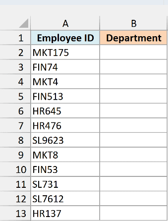
Flash Fill was introduced in Excel 2013.

When you enter an example result in column B, it tries to identify the pattern and give you the result for the other cells in that column.

Here are the steps to get the text part in column B:

1. Select cell B2.

2. Type MKT and press Enter.

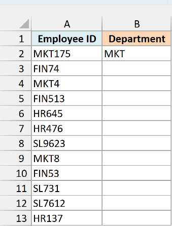
3. With B2 selected again, place the cursor at the bottom-right corner of the cell until it changes to a plus icon.

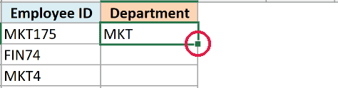
This is called the Fill Handle.

4. Hold the left mouse button and drag the Fill Handle down to B13.

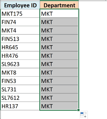
Don’t worry if all the cells are filled with the same text at this point.

5. Click the Auto Fill Options icon that appears beside the filled cells.

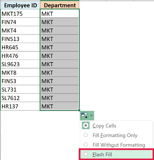
6. Select Flash Fill.

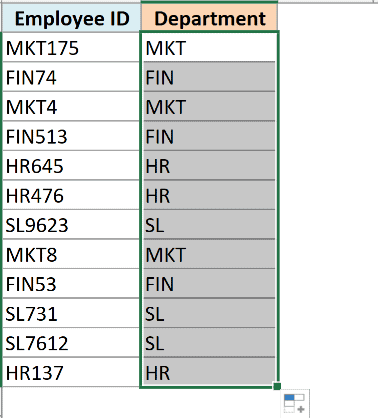
The department codes now appear in B2:B13, with MKT in B2, FIN in B3, and so on.

Pro Tip: After typing MKT in B2, select B3 and press Ctrl+E. Or use Data > Data Tools > Flash Fill.

In Microsoft 365, you may also see grayed-out Flash Fill suggestions while typing the second entry. Press Enter to accept them.

If Flash Fill misreads the pattern, enter the expected result in two or three cells first. Then fill the range and use Flash Fill again.

You can follow the same process for the numbers in column C. Here’s the quicker route:

7. Type 175 in C2 and press Enter.

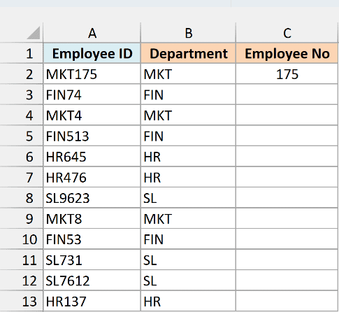
8. Select C3 and press Ctrl+E to fill the remaining employee numbers through C13.

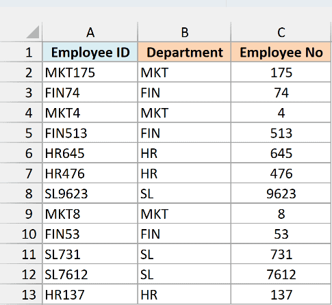
Flash Fill gives you static results. If you change the original data in column A, these results won’t update.

If you want the results to update when the source changes, use the formula method covered next.

Also read: Split Text into Multiple Rows in Excel

Separate Text and Numbers Using Formula

Now let’s look at formulas that update the results when you change the employee IDs.

Below I have IDs such as MKT175, FIN74, and HR645, and I want the department codes in column B and employee numbers in column C.

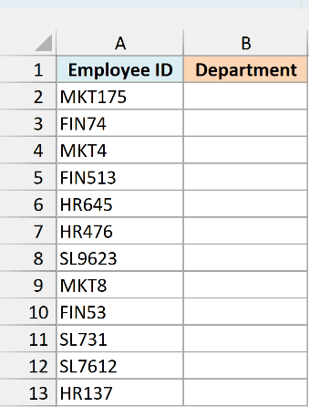
The codes and numbers have different lengths. For example, MKT has three letters, while HR has two.

So the LEFT function alone, with a fixed character count, won’t separate the text correctly.

The same problem applies to extracting the numbers with the RIGHT function.

If you’re using Microsoft 365, use REGEXEXTRACT.

The REGEXEXTRACT function finds the text and number portions using a short pattern.

It’s available in Excel for Microsoft 365 on Windows and Mac, but not Excel 2024, 2021, or older.

Enter this formula in B2 to get the department codes:

=REGEXEXTRACT(A2:A13,"\D+")

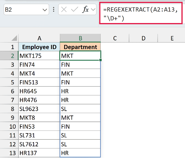
For MKT175, it returns MKT. The formula spills down automatically through B13 and gives you the department code for all 12 employee IDs.

Enter this formula in C2 to get the employee numbers:

=REGEXEXTRACT(A2:A13,"\d+")

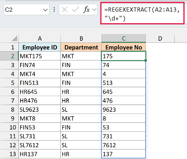
This returns 175 for MKT175 and spills the remaining employee numbers through C13. You don’t need to drag either formula down or use Ctrl+Shift+Enter.

How these formulas work:

• REGEXEXTRACT takes the text to check and a pattern to look for.
• \D matches any character that isn’t a digit, while \d matches a digit.
• The + means one or more matching characters in a row.
• So “\D+” extracts the first run of non-digits, and “\d+” extracts the first run of digits.

You can learn more about these patterns in my tutorial on REGEX functions in Excel.

REGEXEXTRACT always returns text, so the result 175 is text too. That’s useful for employee numbers, especially when you want to keep leading zeros.

If you need numbers for calculations, convert the text with the VALUE function or two minus signs. For example, enter this in C2:

=--REGEXEXTRACT(A2:A13,"\d+")

If there is no match, REGEXEXTRACT returns #N/A. For example, the number formula returns #N/A for a cell containing only ABC.

These formulas also work unchanged when the numbers come first. For 1231ABC, the text formula returns ABC and the number formula returns 1231.

These examples have one text group and one number group. If digits are scattered through your cells, see extracting numbers from a string.

For any Excel version, use LEFT, MID, and FIND.

If REGEXEXTRACT isn’t available in your version, you can find where the first digit starts and split the cell at that position.

Below I have the same employee IDs, and this time I want to use formulas to get the department codes in column B and the employee numbers in column C.

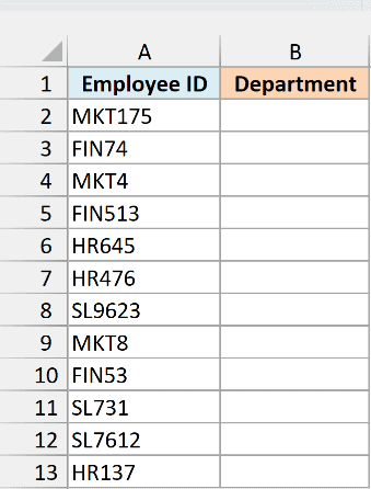
Enter this formula in B2 to extract the text from the left:

=LEFT(A2,MIN(FIND({0,1,2,3,4,5,6,7,8,9},A2&"0123456789"))-1)

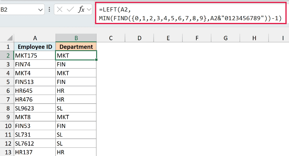
It returns MKT for the employee ID MKT175.

Enter this formula in C2 to extract the numbers:

=MID(A2,MIN(FIND({0,1,2,3,4,5,6,7,8,9},A2&"0123456789")),LEN(A2))

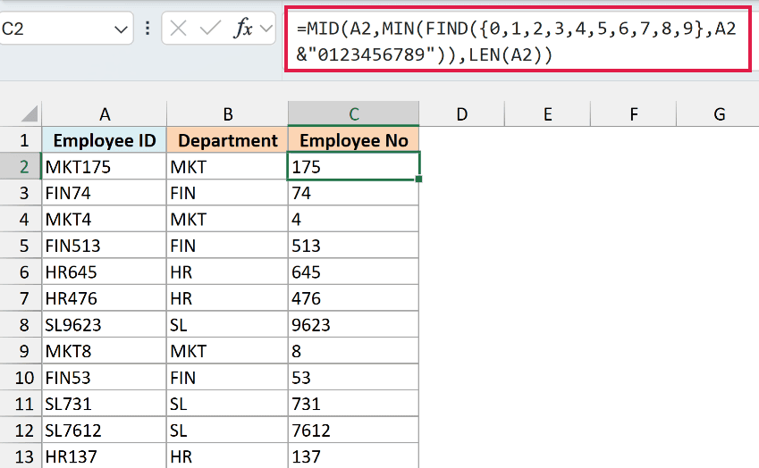
This returns 175. Copy the formulas down through B13 and C13 to separate all the employee IDs.

Both are normal formulas in every Excel version. Unlike the IFERROR version you may have seen, they don’t need Ctrl+Shift+Enter in older Excel.

How this formula works:

Let me first explain the formula that we use to separate the text part on the left.

• A2&”0123456789″ adds all ten digits to the end of the cell’s contents. For MKT175, the text being searched becomes MKT1750123456789.
• The FIND function looks for the first occurrence of each digit from 0 to 9 in that combined text.
• It returns {7,4,9,10,11,6,13,5,15,16}. Each number is the position of the corresponding digit.
• For 0, it returns 7 because the first 0 is in the appended digits. For 1, it returns 4 because the first 1 is already in MKT175. And so on.
• The MIN function takes the smallest position, which is 4. This tells us where the first digit starts.
• LEFT then takes everything before that position. LEFT(A2,4-1) returns the first three characters, MKT.

Normally, FIND returns a #VALUE! error when it can’t find a character.

Appending all ten digits means FIND always finds each one, so there’s no missing-digit error to handle.

To get the numbers, the MID function uses the same starting position.

For MKT175, MID starts at position 4 and requests LEN(A2) characters, which is enough to take everything through the end. The result is 175.

If A2 contains only ABC, the first digit is found after the original text ends. LEFT returns ABC, and MID returns an empty result.

These formulas return text too. If you need to calculate with the employee numbers, convert the extracted values to numbers.

If you replace A2 with A2:A13, the MIN function combines positions across the rows, so it won’t find the first digit separately for each ID.

That’s why you should keep these formulas separate for each row, even in Microsoft 365.

And what if the numbers come first?

If you’re using Microsoft 365, the REGEXEXTRACT formulas above already handle this.

For older versions, we can count the digits and use that count to separate the number from the text.

Below I have employee IDs with numbers first, such as 175MKT and 74FIN, and I want the numbers in column B and department codes in column C.

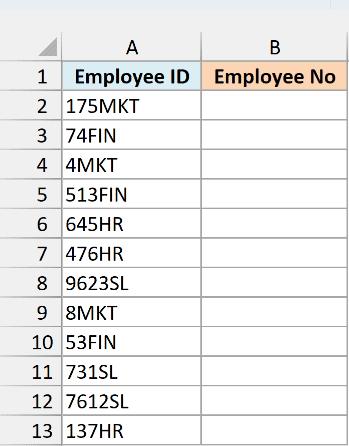
Enter this formula in B2 to get the employee number:

=LEFT(A2,SUM(LEN(A2)-LEN(SUBSTITUTE(A2,{0,1,2,3,4,5,6,7,8,9},""))))

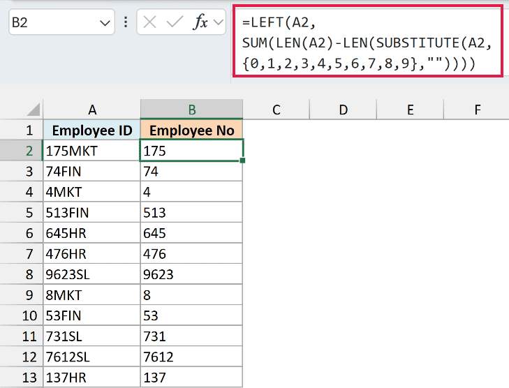
For 175MKT, it returns 175.

Enter this formula in C2 to get the department code:

=MID(A2,SUM(LEN(A2)-LEN(SUBSTITUTE(A2,{0,1,2,3,4,5,6,7,8,9},"")))+1,LEN(A2))

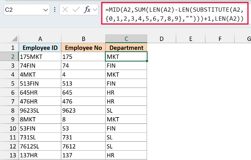
It returns MKT. Copy both formulas down through row 13.

How these formulas work:

• SUBSTITUTE removes each digit from the text in turn.
• LEN counts the characters before and after each removal. The difference tells us how many times that digit appears.
• SUM adds those counts. For 175MKT, the total digit count is 3.
• LEFT takes the first three characters, 175. MID starts at the next character, position 4, and returns MKT.

Important: All digits must be together at the start. A stray digit later, as in 175MKT2, gives a wrong split without an error.

Separate Text and Numbers Using VBA (Custom Function)

If you need to do this quite often, you can create your own custom function using VBA.

Each function takes just one argument, the cell reference, so it’s easier to use than the longer formulas.

Below I have employee IDs, and I want the department codes in column B and the employee numbers in column C.

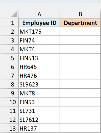
The download file already contains these functions. If you want to add them to another workbook, use the code and steps below.

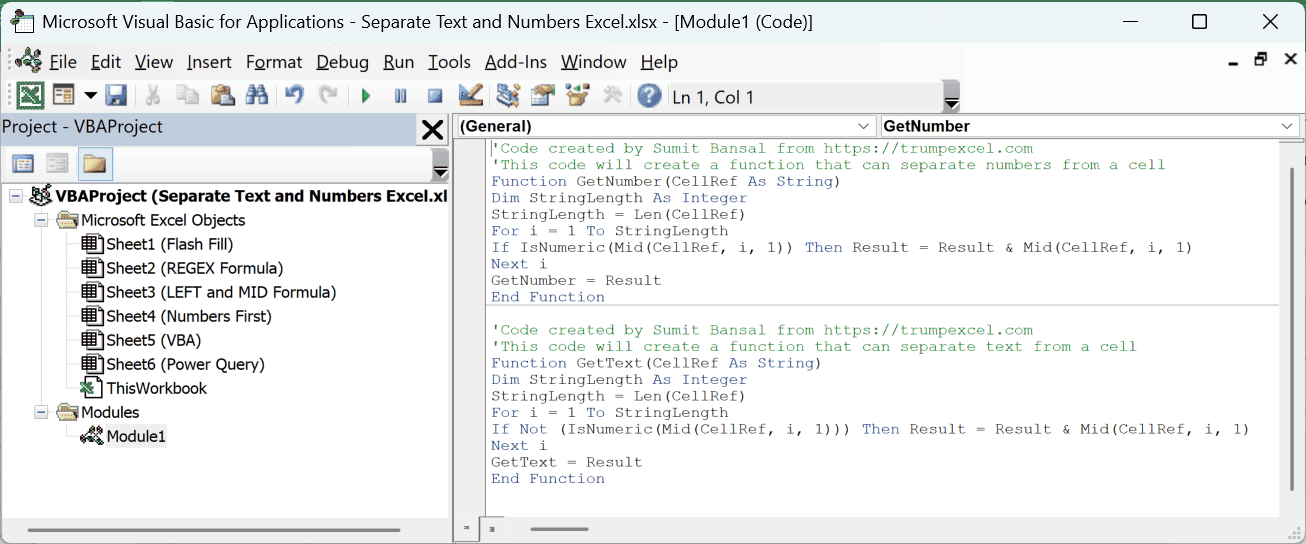
This code creates GetNumber, which goes through the cell one character at a time and keeps each digit:

'Code created by Sumit Bansal from https://trumpexcel.com
'This code will create a function that can separate numbers from a cell
Function GetNumber(CellRef As String)
Dim StringLength As Integer
StringLength = Len(CellRef)
For i = 1 To StringLength
If IsNumeric(Mid(CellRef, i, 1)) Then Result = Result & Mid(CellRef, i, 1)
Next i
GetNumber = Result
End Function

'Code created by Sumit Bansal from https://trumpexcel.com'This code will create a function that can separate numbers from a cellFunction GetNumber(CellRef As String)Dim StringLength As IntegerStringLength = Len(CellRef)For i = 1 To StringLengthIf IsNumeric(Mid(CellRef, i, 1)) Then Result = Result & Mid(CellRef, i, 1)Next iGetNumber = ResultEnd Function

And this code creates GetText, which keeps each character that isn’t a digit:

'Code created by Sumit Bansal from https://trumpexcel.com
'This code will create a function that can separate text from a cell
Function GetText(CellRef As String)
Dim StringLength As Integer
StringLength = Len(CellRef)
For i = 1 To StringLength
If Not (IsNumeric(Mid(CellRef, i, 1))) Then Result = Result & Mid(CellRef, i, 1)
Next i
GetText = Result
End Function

'Code created by Sumit Bansal from https://trumpexcel.com'This code will create a function that can separate text from a cellFunction GetText(CellRef As String)Dim StringLength As IntegerStringLength = Len(CellRef)For i = 1 To StringLengthIf Not (IsNumeric(Mid(CellRef, i, 1))) Then Result = Result & Mid(CellRef, i, 1)Next iGetText = ResultEnd Function

Here are the steps to add both functions to your workbook:

1. Click the Developer tab in the ribbon.

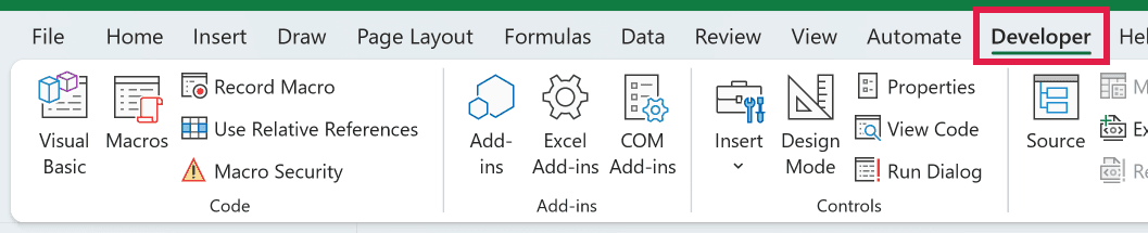
2. Click Visual Basic to open the editor.

You can also press Alt+F11 to open the Visual Basic Editor.

Project Explorer on the left shows your workbook and its worksheets. If it’s hidden, use the following step; otherwise, skip to step 4.

3. Choose View > Project Explorer.

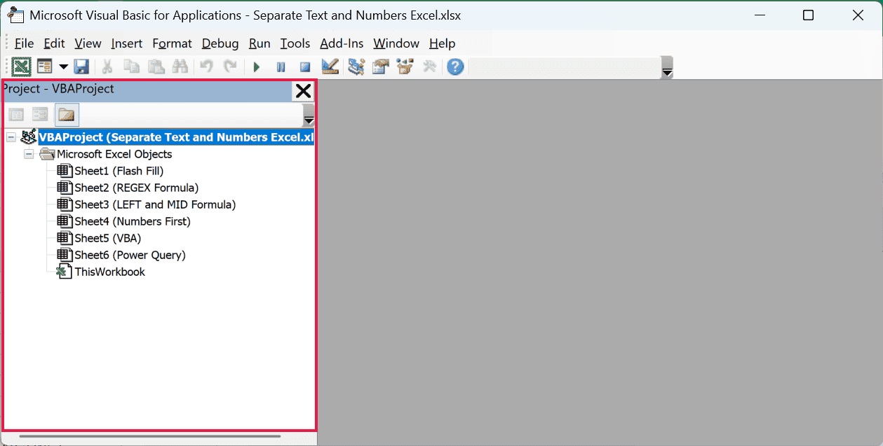
4. Select any worksheet name or other object under the workbook where you want to add the functions.

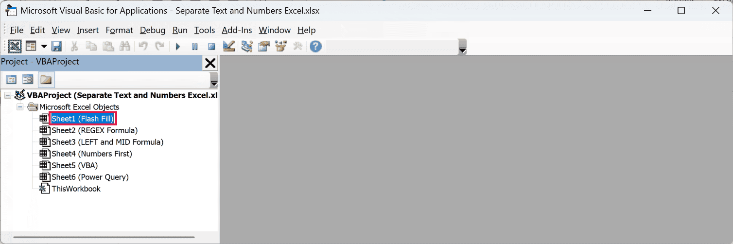
5. Choose Insert > Module.

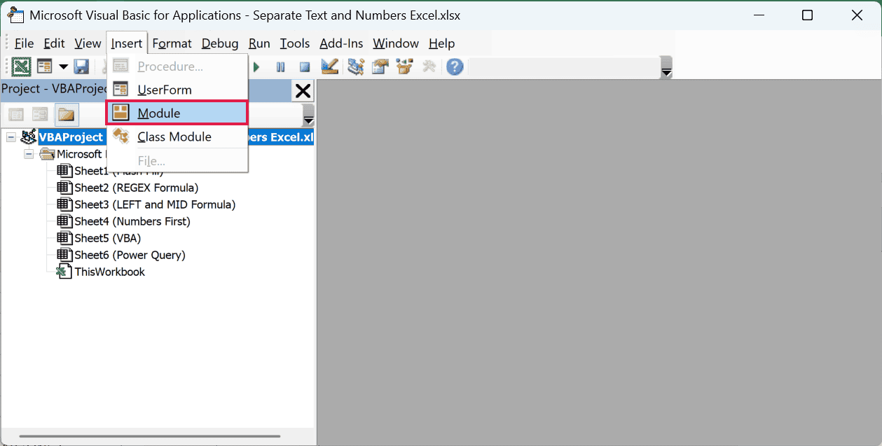
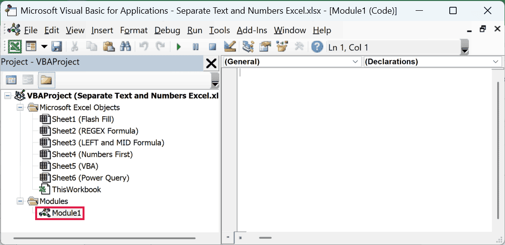
A new module is added, and its code window opens. If it doesn’t open, use this optional step:

6. Double-click the new module in Project Explorer to open its code window.

7. Paste both functions into the module code window.

8. Close the VB Editor.

You can now use these functions just like other worksheet functions.

9. Save the workbook as an Excel Macro-Enabled Workbook (.xlsm).

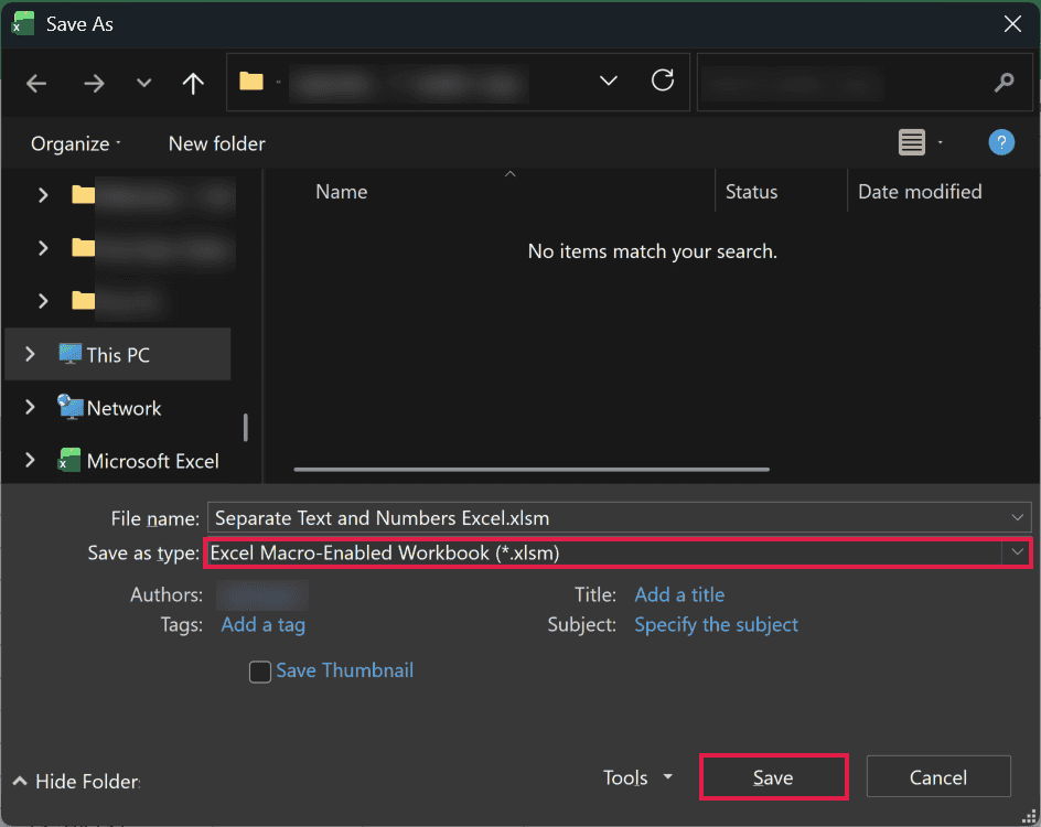
The .xlsm format keeps the VBA code. Saving as .xlsx won’t retain it.

Enter this formula in B2 to get the department code:

=GetText(A2)

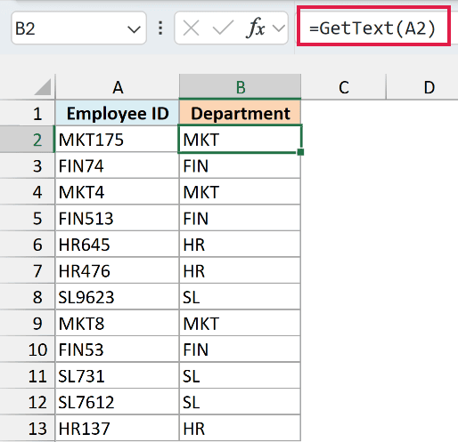
It returns MKT for MKT175.

Enter this formula in C2 to get the employee number:

=GetNumber(A2)

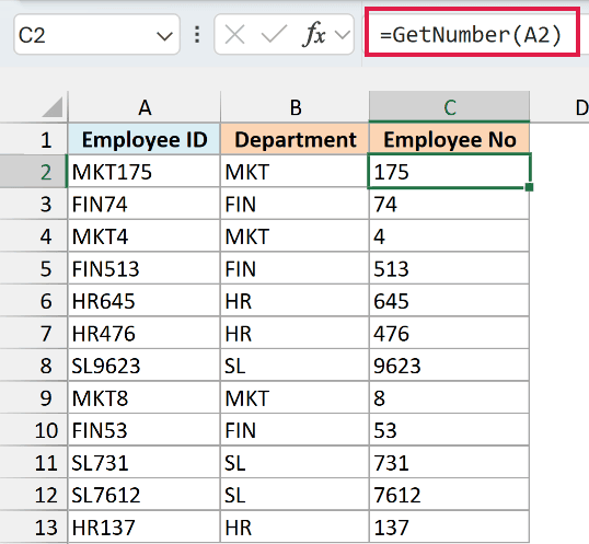
It returns 175. Copy the formulas down through B13 and C13.

GetNumber returns the digits as text. Unlike the formulas above, it collects every digit in the cell, wherever it sits.

If you do this often, you can save both functions in your Personal Macro Workbook.

That makes them available in other workbooks on your system, so you don’t need to add the code to each workbook.

When a function is stored there, prefix its name with PERSONAL.XLSB!. For example:

=PERSONAL.XLSB!GETNUMBER(A2)

Separate Text and Numbers Using Power Query

Power Query is slowly becoming my favorite feature in Excel.

If you’re already using Power Query as part of your workflow, it can separate the text and numbers in a few clicks.

Below I have employee IDs in the EmployeeData table, and I want to split them into Department and Employee No columns.

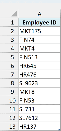
Power Query needs the source data in an Excel Table.

You can also use a named range, but we’re using a table in this example.

Here are the steps:

1. Select any cell in the EmployeeData table.

2. Click the Data tab.

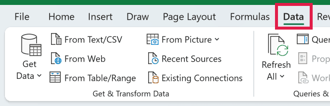
3. In the Get & Transform Data group, click From Table/Range.

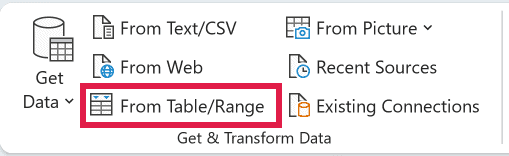
If your data isn’t already a table, Excel shows the Create Table dialog. Confirm the range and headers to convert it into a table.

4. In the Power Query editor, select the Employee ID column.

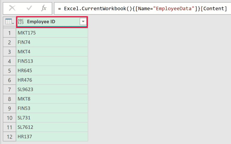
5. Click the Transform tab.

6. Click Split Column.

You can also find Split Column on the Home tab.

7. Select By Non-Digit to Digit.

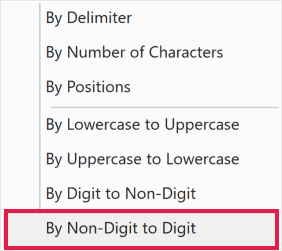
The column splits into Employee ID.1 (the department codes) and Employee ID.2 (the employee numbers).

This option splits at every change from a non-digit to a digit. For numbers-first IDs such as 175MKT, use By Digit to Non-Digit instead.

You can optionally rename the columns to make the output easier to read:

8. Double-click the Employee ID.1 header and rename it Department.

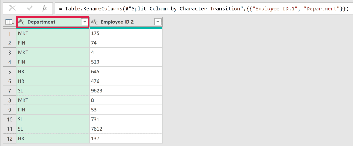
9. Double-click the Employee ID.2 header and rename it Employee No.

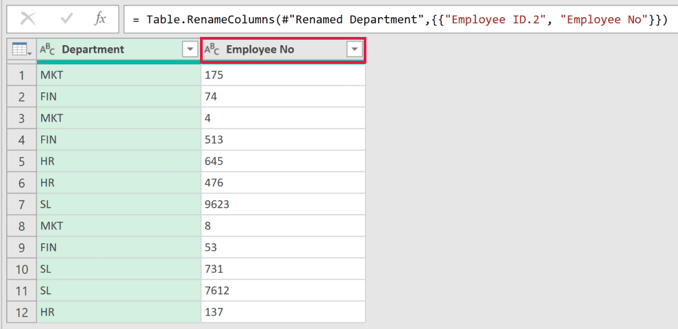
Employee No comes out as text. If you need real numbers, you can click the ABC icon in its column header and pick Whole Number.

Converting to Whole Number drops any leading zeros. The example file keeps Employee No as text.

10. Click the Home tab in the Power Query editor.

11. Click Close & Load.

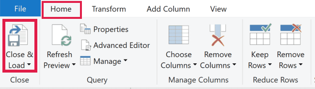
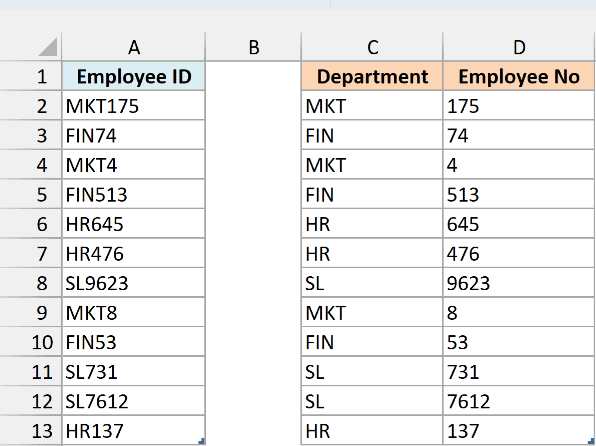
By default, this loads the output as a table on a new worksheet.

In the example file, I used Close & Load To to place the result at C1:D13 next to the source, so both tables are visible.

Now let me tell you the best part about this method.

Your original Excel Table (the data source) stays connected to the output table.

So if you change the original data, you don’t need to repeat the entire process. To update the results:

12. Right-click any cell in the result table and choose Refresh.

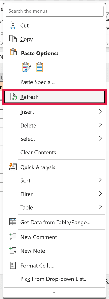
You can also use Data > Refresh All.

Power Query checks the original source, runs the same transformations, and updates the output.

This is where Power Query really shines.

It remembers every step you took, so you can set up a transformation once and reuse it whenever you need it.

When you get new data, put it in place of the old data in the source table and refresh the query. You’ll get the updated results in a few seconds.

Alternatively, you can change the query’s source to another Excel Table in the same workbook or a different workbook.

So these are four simple ways you can use to separate numbers and text in Excel. If this is a once-in-a-while activity, you’re better off using Flash Fill or the formula method.

And in case this is something you need to do quite often, then I would suggest you consider the VBA method where we created a custom function or the Power Query method.

I hope you found this Excel tutorial useful.

Other Excel tutorials you may also like:

• Separate First and Last Name in Excel (Split Names Using Formulas)
• How to Convert Numbers to Text in Excel
• Convert Text to Numbers in Excel – A Step By Step Tutorial
• How to Compare Text in Excel
• How to Quickly Combine Cells in Excel
• How to Combine First and Last Name in Excel
• How to Extract the First Word from a Text String in Excel (3 Easy Ways)
• Extract Numbers from a String in Excel (Using Formulas or VBA)
• How to Extract a Substring in Excel (Using TEXT Formulas)
• REGEX Functions in Excel
• Remove Characters From Left in Excel (Easy Formulas)