Show Negative Numbers in Parentheses (Brackets) in Excel (Easy Ways)

When you’re preparing a profit or finance report, you might want negative numbers in parentheses, but Excel shows them with a minus sign by default.

For example, if you type -182029, Excel shows -182029 even though your report needs (182029).

There are a few ways to fix this: the built-in Format Cells option, Accounting format, or a custom number format.

I’ll show you each method and how to restore the parentheses option if it’s missing.

Show Negative Numbers in Parentheses Using Format Cells

Excel already has some inbuilt number formats that will show the negative number in brackets.

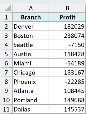
Below I have a data set where I have the profit values for different branches in column B, and I want to show the negative values in brackets.

Here are the steps to do this:

1. Select the cells that have the numbers (you can select the entire range of cells, not just the negative numbers)

2. Click the ‘Home’ tab

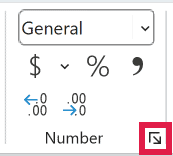
3. In the ‘Number’ group, click on the dialog box launcher icon (small arrow at the bottom right part of the group)

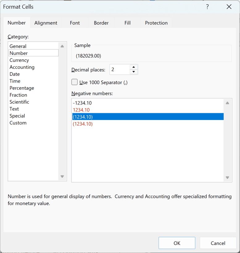
4. In the ‘Format Cells’ dialog box, within the ‘Number’ tab, make sure ‘Number’ is selected in the Category list

5. Select the third option in the Negative numbers list (the one that shows the number in the bracket as is in black color)

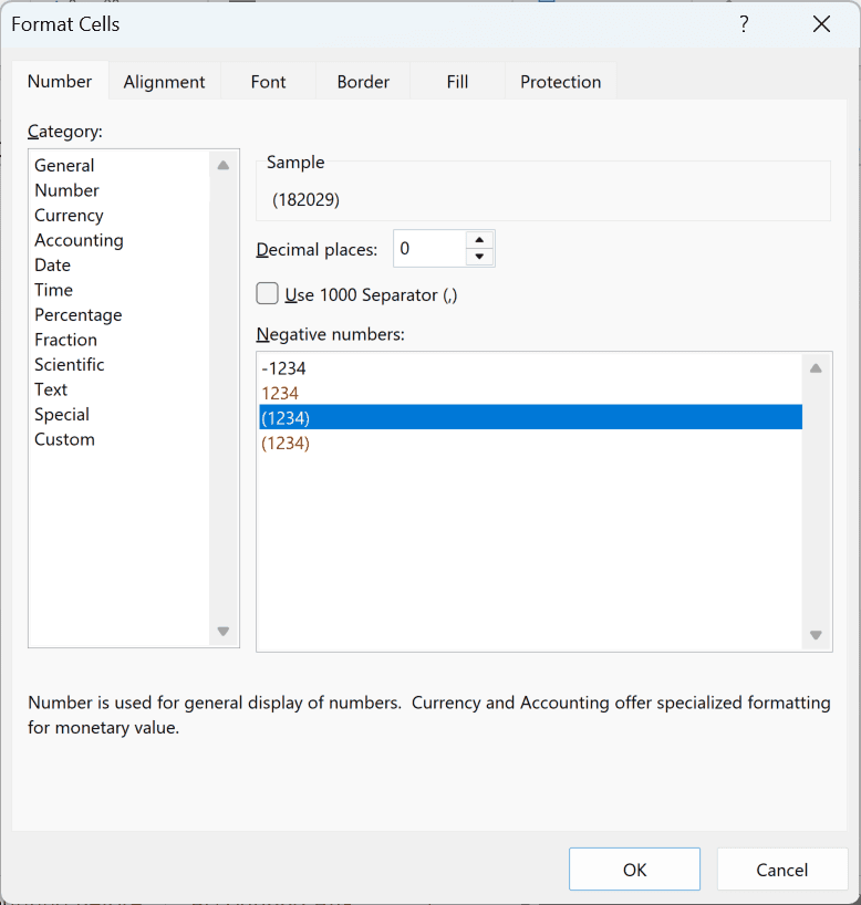
6. [Optional] Specify the decimal numbers you want to show. In case you don’t want decimal numbers, make the value 0 (it’s 2 by default)

7. Click OK

The above steps would change the format of the cells so that the negative numbers are now shown within parentheses (as shown below).

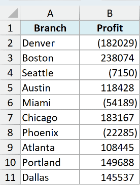
Note that this only changes how the numbers look. The actual values in the cells stay the same, so any calculations using these cells are not affected.

Pro Tip: You can also use the keyboard shortcut Ctrl+1 to open the Format Cells dialog box directly.

In the ‘Format Cells’ dialog box, you also get the option to have the negative numbers in brackets as well as change the color of these negative numbers to Red.

If you want to show negative numbers in red color within brackets, select the fourth option in step 5.

Important: There is a possibility that you may not see the same ‘Negative numbers’ formatting options as I’ve shown in the screenshots above.

Some systems have settings where it does not show the option to format negative numbers to show them in brackets.

Instead, it shows the options with the minus sign.

In such a case, you will have to change your system settings (as <a href=”#Fix-a-Missing-Parentheses-Option-in-Excel”>covered later in this tutorial</a>).

Also read: How to Make Negative Numbers Show Up in Red in Excel

Show Negative Numbers in Parentheses with Accounting Number Format

If you’re working with currency values, the Accounting Number Format is another quick option.

It adds the currency symbol, shows negative numbers in brackets, and lines up the decimal points in the column.

Below I have the same data set with the profit values for different branches, and I want to show these as dollar values with the negative values in brackets.

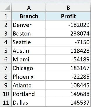
Here are the steps to do this:

1. Select the cells that have the numbers

2. Click the ‘Home’ tab

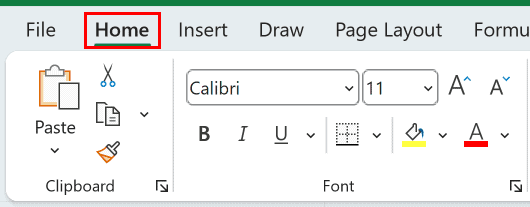
3. In the ‘Number’ group, click on the Accounting Number Format button (the one with the dollar sign)

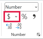
That’s it! Denver’s profit is now shown as $ (182,029.00), while Boston’s profit is shown as $ 238,074.00.

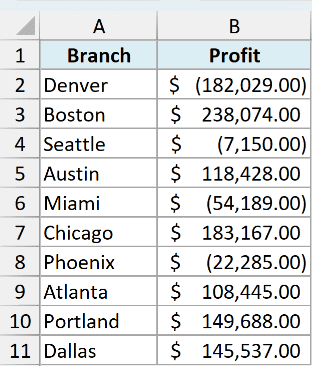
Important: The brackets come from your Windows regional settings. If you see a minus sign instead, use a custom format or change your system settings.

Show Negative Numbers in Parentheses with a Custom Format

While the above methods do allow you to show negative numbers in brackets (in black or red color), you may need more control on how these numbers should be shown.

In such a case, you can create your own custom number format.

For example, you may want to show the negative numbers in brackets along with a minus sign (or show them in orange/brown color instead of red).

Below I have a data set where I have the profit values for different branches, and I want to show the negative numbers in brackets (with a comma as the thousands separator).

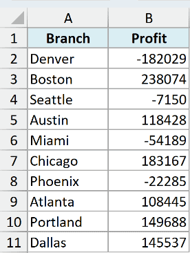
Below are the steps to do this:

1. Select the cells that contain the negative numbers that you want to format

2. Click the ‘Home’ tab

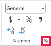
3. In the ‘Number’ group, click on the dialog box launcher

4. In the ‘Format Cells’ dialog box, within the ‘Number’ tab, select the ‘Custom’ option

5. In the ‘Type’ field, enter the below custom format: #,##0;(#,##0)

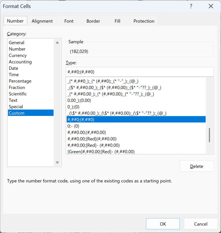
6. Click OK

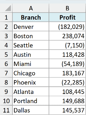
The above steps would change the formatting of the cells, and the negative numbers would now be shown in brackets.

So Denver’s profit is shown as (182,029), and Boston’s profit is shown as 238,074.

Let me quickly explain how custom number formatting works, and then I will give you some examples of other formats you can use.

In Excel, you can enter the following types of data:

• Positive Number
• Negative Number
• Zero
• Text

For any cell, you can specify the format for any of the above data types.

This means that I can specify how the positive numbers should be shown in a cell, how the negative numbers should be shown, and how zero and text values should be shown.

And below is how the custom number format should be created:

<Format for Positive Number>;<Format for Negative Number>;<Format for Zero>;<Format for Text>

Note that each of these formats is separated by a semi-colon.

You don’t have to specify all four formats. If you only specify two (as we did above), the first one is used for positive numbers as well as zero.

The second one is used for negative numbers, and any text is shown as it is.

In our example, we used the format <code>#,##0;(#,##0)</code>

Where:

• Positive Number format – <code>#,##0</code> – This means that the number is shown with a thousands separator and no decimals (so 1234.5 would be shown as 1,235)
• Negative Number format – <code>(#,##0)</code> – This means that the number is shown in the same way, but within parentheses
• Zero format – since this is not specified, the positive number format is used
• Text format – since this is not specified, the text is shown as it is

In case you want to show the negative numbers in brackets along with a minus sign, you can use the below format:

0;- (0)

With this format, any negative number would be displayed in a bracket with a negative sign outside the bracket. So -1234.5 would be shown as – (1235).

Note that the 0 in this format code rounds the number to a whole number, which is why 1234.5 shows up as 1235 (the value in the cell doesn’t change).

Now that you have a basic understanding of how custom number formatting works in Excel, here are some more formats that you can use:

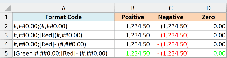
Showing the numbers with thousand separators, and negative numbers in parentheses

#,##0.00;(#,##0.00)

Showing the negative numbers in red color and in parentheses

#,##0.00;[Red](#,##0.00)

Showing the negative numbers in red color and in parentheses with a minus sign

#,##0.00;[Red]- (#,##0.00)

Showing the negative numbers in red color and positive numbers in green color

[Green]#,##0.00;[Red]- (#,##0.00)

Below you can see how each of these formats shows a positive number, a negative number, and zero.

In case you want to use a color other than red or green (such as orange or brown), you can use a color number instead of the color name.

For example, [Color46] gives you orange and [Color53] gives you brown:

#,##0;[Color46](#,##0)

Along with color numbers from [Color1] to [Color56], you can use eight color names in a custom format: [Black], [Blue], [Cyan], [Green], [Magenta], [Red], [White], and [Yellow].

The zero section of a custom format can also be used to hide zero values in cells.

Also read: Remove Parentheses in Excel

Line Up Positive Numbers with Bracketed Negatives

When you show negative numbers in brackets, you may notice that the positive numbers don’t line up perfectly with the negative numbers.

This is because the closing bracket takes up a little extra space.

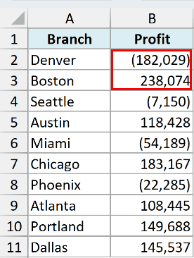
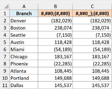
Below I have a data set where the profit values use the format <code>#,##0;(#,##0)</code>. If you look closely, the last digit of 238,074 sits a little to the right of the last digit of (182,029).

I want the last digits of all the numbers to line up (such that 9 in cell B2 aligns with 4 in cell B3).

To do this, you can add <code>_)</code> after the positive number format.

The underscore tells Excel to add a space as wide as the character that follows it, which in this case is the closing bracket.

Here are the steps to do this:

1. Select the cells that have the profit values

2. Hold the Control key and press 1 to open the Format Cells dialog box

3. Within the ‘Number’ tab, select the ‘Custom’ option

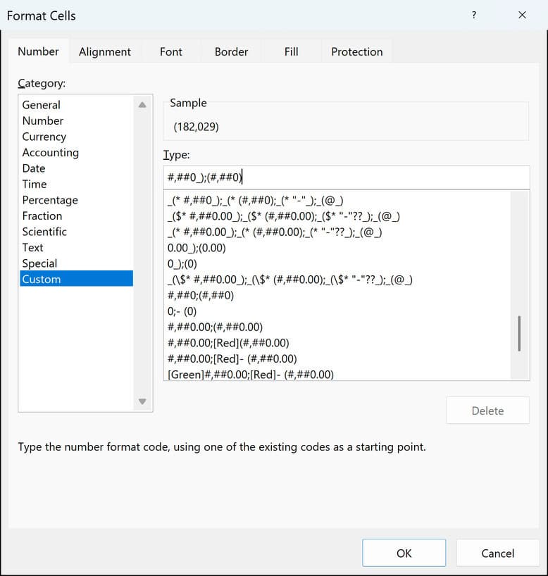
4. In the ‘Type’ field, enter the below custom format: #,##0_);(#,##0)

5. Click OK

Now the positive numbers get a small space on the right, so they line up with the negative numbers in brackets.

Below you can see both formats side by side. The column on the left uses the original format, and the column on the right uses the new one with <code>_)</code>.

In fact, this is exactly what the built-in format we used in the first method does.

If you check its custom code, you would see <code>0_);(0)</code>.

And in case you use two decimal places and a thousands separator, you would see <code>#,##0.00_);(#,##0.00)</code>.

Show Negative Percentages in Parentheses

The built-in Percentage format in Excel doesn’t have an option to show negative percentages in brackets. But you can easily do this with a custom format.

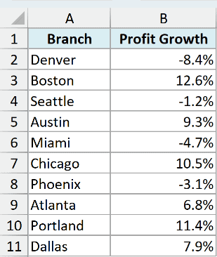
Below I have a data set where I have the profit growth percentage for different branches, and I want to show the negative percentages in brackets.

Here are the steps to do this:

1. Select the cells that have the percentages

2. Hold the Control key and press 1 to open the Format Cells dialog box

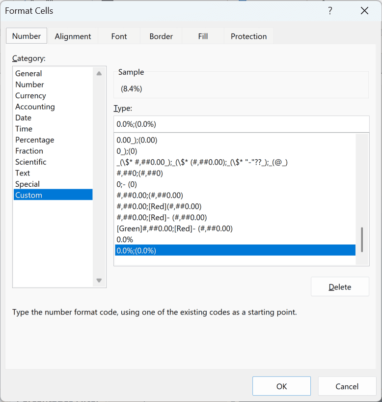
3. Within the ‘Number’ tab, select the ‘Custom’ option

4. In the ‘Type’ field, enter the below custom format: 0.0%;(0.0%)

5. Click OK

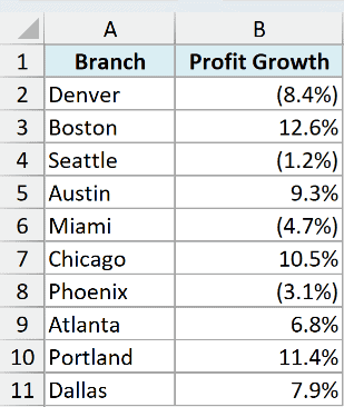
The above steps would show the negative percentages in brackets. So Denver’s growth of -8.4% is now shown as (8.4%), while Boston’s growth is still shown as 12.6%.

In case you want two decimal places, you can use <code>0.00%;(0.00%)</code> instead.

Fix a Missing Parentheses Option in Excel

When you open the Format Cells dialog box and select the Number option, you should see the option to show negative numbers in brackets.

But on some systems, you would only see the options with the minus sign (as shown below).

In case you don’t see these options, it could be because of the settings in your system.

Here is how you can change the settings so it shows you the options to format cells so that negative numbers are shown within parentheses:

1. Close Excel

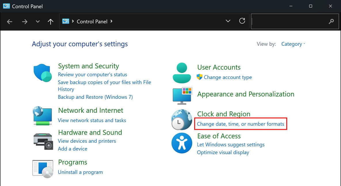
2. Open Control Panel on your system (make sure ‘View by’ is set to Category)

3. Under Clock and Region, click on the ‘Change date, time, or number formats’ option

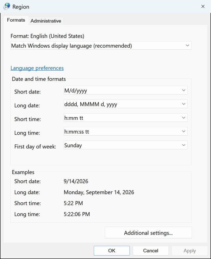
4. In the Region dialog box, within the ‘Formats’ tab, click on the ‘Additional settings’ button

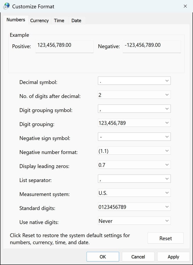
5. In the Numbers tab, change the ‘Negative number format’ to (1.1) from the drop-down

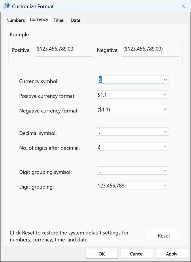
6. In the Currency tab, change the ‘Negative currency format’ to ($1.1) from the drop-down

7. Click OK

8. Click OK

9. Open Excel again

The above steps would change your system’s setting and you will be able to see the formatting option to show negative numbers in brackets in the Format Cells dialog box.

Pro Tip: You can also open the Region dialog box directly. Press Windows key + R, type intl.cpl, and press Enter.

Important: This is a Windows setting, so it also changes how negative numbers and currency values are shown in other applications.

In case you don’t want to change it, you can use the custom number format method instead, as it works on any system.

In this tutorial, I showed you how to change the format of the cells to show negative numbers in brackets.

I also covered how you can customize the format to add a minus sign along with the brackets as well as change the color of the negative numbers.

Along with that, I showed you the Accounting format, how to line up positive and negative numbers, and how to show negative percentages in brackets.

And in case the option to show negative numbers in brackets is missing, I also showed you how to fix it by changing your system settings.

I hope you found this tutorial useful.

Other articles you may also like:

• How to Sum Only Positive or Negative Numbers in Excel (Easy Formula)
• <a href=”https://trumpexcel.com/change-negative-to-positive-in-excel/”>Change Negative Number to Positive in Excel [Remove Negative Sign]</a>
• Color Negative Chart Data Labels in Red with a downward arrow
• How to Sum by Color in Excel (Formula & VBA)
• How to Remove Cell Formatting in Excel (from All, Blank, Specific Cells)
• How to Filter Cells with Bold Font Formatting in Excel
• How to Display Numbers as Fractions (Write Fractions in Excel)
• Add Parentheses Around Text in Excel
• Format Numbers to Show in Millions in Excel
• Hide Zero Values in Excel | Make Cells Blank If the Value is 0
• How to Add Plus Sign Before Numbers in Excel