

If you want to average only the numbers that meet more than one condition, a plain AVERAGE won’t get you there. It averages everything in the range, with no way to say “only these rows.”
That’s exactly what the AVERAGEIFS function is for. You give it a range of numbers to average, then pair up as many criteria as you need, and it averages only the rows where every condition is true.
In this article, I’ll show you how to use AVERAGEIFS with two or more criteria, comparison operators, date ranges, and wildcards. I’ll also show you how to handle OR logic and the #DIV/0! error when nothing matches.
Follow along with the example file
AVERAGEIFS Function Examples.xlsx
AVERAGEIFS Syntax and Arguments
Here is the syntax of the AVERAGEIFS function:
=AVERAGEIFS(average_range, criteria_range1, criteria1, [criteria_range2, criteria2], ...)
- average_range – the range of numbers you actually want to average.
- criteria_range1 – the first range Excel checks a condition against.
- criteria1 – the condition applied to criteria_range1 (a number, text, or an expression like “>100”).
- [criteria_range2, criteria2] – optional extra range and condition pairs. AVERAGEIFS accepts up to 127 pairs in total, including the first required pair.
The one thing to burn into memory: average_range comes first, before any criteria. This trips people up because AVERAGEIF (the single-criterion version) puts the average range last. AVERAGEIFS flips it to the front, the same way SUMIFS does.
Every criteria_range has to be the same size and shape as average_range. If average_range is 12 rows, each criteria_range needs to be the same 12 rows.
Pro Tip: Text criteria and any criteria using an operator (like “>100” or “<>Laptop”) must be wrapped in double quotes. Plain numbers like 100 don’t need quotes.
Example 1: Average With Two or More Criteria
Let’s start with the most common use of AVERAGEIFS: averaging with two conditions at once.
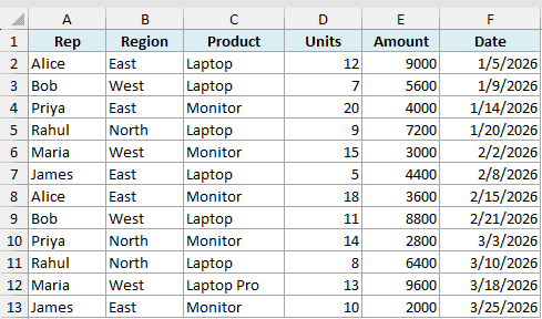
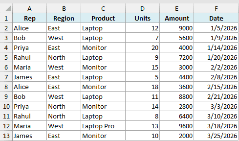
Below is a sales dataset. Column A has the rep, column B the region, column C the product, column D units sold, column E the sale amount, and column F the date. I want the average sale amount for laptops sold in the East region.
Here is the formula:
=AVERAGEIFS(E2:E13, B2:B13, "East", C2:C13, "Laptop")
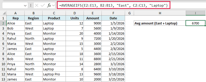
This returns 6700. Excel looks down the region column for “East” and the product column for “Laptop”, finds the two rows where both are true, and averages their amounts (9000 and 4400).
The pattern is always the same. The range you’re averaging goes first, then each condition is a range/criteria pair. Add a third pair and Excel narrows it further, keeping only rows where all three are true. It’s the same multiple-criteria logic COUNTIFS and SUMIFS use.
Example 2: Average Using Comparison Operators (Greater Than, Less Than)
Now let’s use a criterion that isn’t an exact match. Comparison operators like >, <, >=, and <> let you average based on a threshold instead of a fixed value.
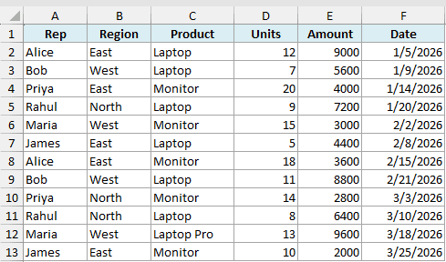
Same sales dataset as before. This time I want the average sale amount for orders of at least 10 units, using the units column in D.
Here is the formula:
=AVERAGEIFS(E2:E13, D2:D13, ">=10")
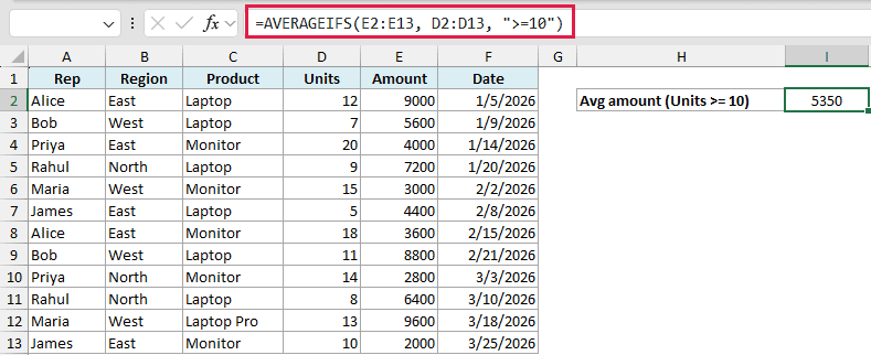
This returns 5350, the average amount across the eight rows where units are 10 or more. Note the whole condition ">=10" sits inside double quotes, operator and number together.
If your threshold lives in a cell instead of being typed in, join the operator to the cell reference with an ampersand. So ">="&H1 reads the number from H1. Only the operator goes in quotes here, not the cell reference.
Example 3: Average Between Two Dates
A common task is averaging values that fall inside a date window. You do this with two criteria on the same date column: one for the start date and one for the end date.
Using the same dataset, I want the average sale amount for orders placed in February 2026, between the 1st and the 28th. The dates are in column F.
Here is the formula:
=AVERAGEIFS(E2:E13, F2:F13, ">="&DATE(2026,2,1), F2:F13, "<="&DATE(2026,2,28))
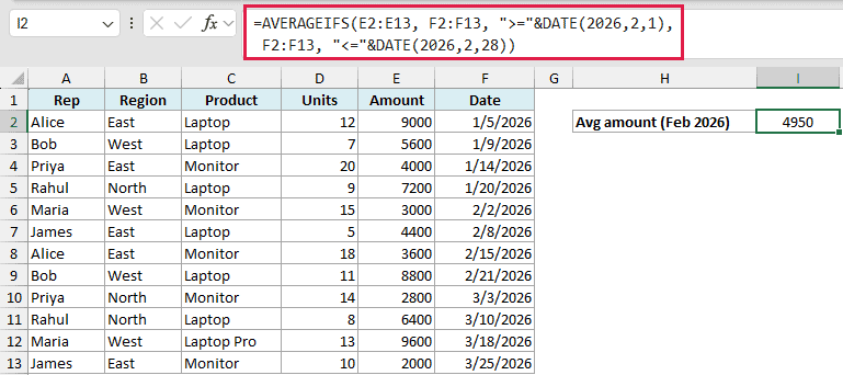
This returns 4950, the average of the four February orders. The same date column F2:F13 is used twice, once with an “on or after the 1st” condition and once with an “on or before the 28th” condition.
I’m using DATE(2026,2,1) instead of typing “2/1/2026” so Excel reads it as a real date no matter what regional format your machine uses. It’s the safer way to feed a date into a criterion.
Important: Times after midnight on February 28 are excluded. Use "<"&DATE(2026,3,1) as the upper condition to include the whole day.
Example 4: Average Using Wildcards (Partial Text Match)
AVERAGEIFS accepts wildcard characters in text criteria, so you can match on part of a word instead of the whole thing. The asterisk * stands for any number of characters, and the question mark ? stands for exactly one character.
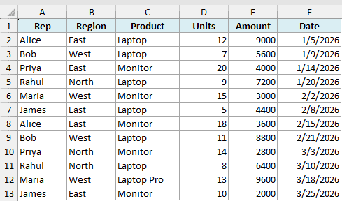
Same dataset again. Say the product column has entries like “Laptop” and “Laptop Pro”, and I want every product that starts with “Lap” sold in the West region. I’ll match on "Lap*".
Here is the formula:
=AVERAGEIFS(E2:E13, B2:B13, "West", C2:C13, "Lap*")
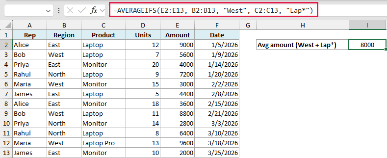
This returns 8000, the average amount of the three West-region rows whose product starts with “Lap”. The * after “Lap” tells Excel to accept anything that follows.
If you ever need to match a literal asterisk or question mark, put a tilde in front of it (~* or ~?) so Excel treats it as a real character instead of a wildcard.
Example 5: Handling the #DIV/0! Error When Nothing Matches
Here’s the gotcha that catches people. When no rows meet all your criteria, AVERAGEIFS has nothing to average, so it returns a #DIV/0! error rather than a blank or a zero.
Using the same sales data, suppose I ask for the average amount in the “South” region. There are no South rows in the data at all.
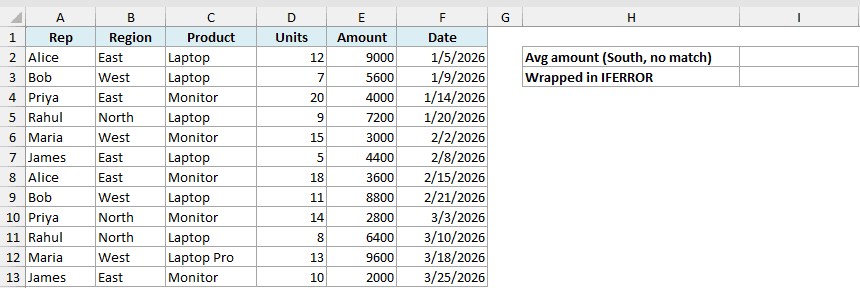
Here is the formula:
=AVERAGEIFS(E2:E13, B2:B13, "South")
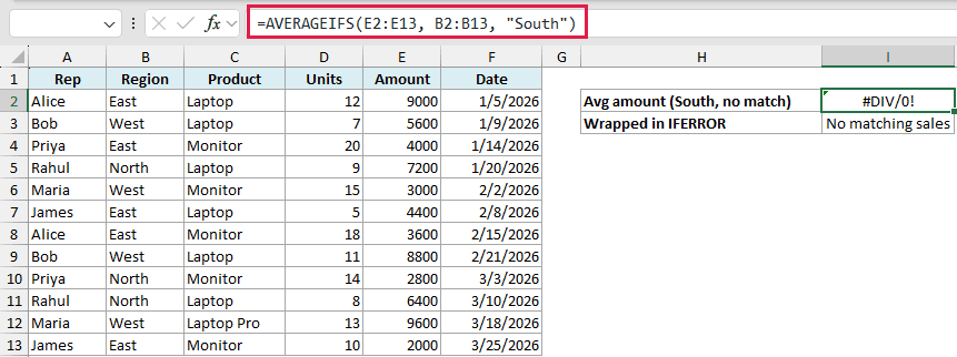
Because nothing matches, this returns #DIV/0! instead of a number. To show a friendly message instead of the error, wrap the whole thing in IFERROR.
Here is the formula:
=IFERROR(AVERAGEIFS(E2:E13, B2:B13, "South"), "No matching sales")
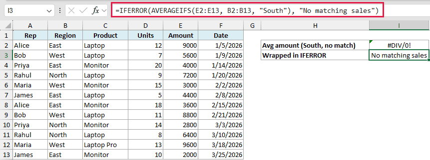
Now the cell shows “No matching sales” when nothing matches. IFERROR also replaces other errors with this message, so check the underlying formula before relying on the result.
Pro Tip: AVERAGEIFS also throws #DIV/0! if none of the matched rows has a numeric value in average_range. Text or blanks mixed with numbers don’t cause this error.
Example 6: Get an Average Per Category in One Formula (Excel 365, 2024, or 2021)
All the examples above return a single value. In Excel 365, 2024, 2021, or Excel for the web, you can get an average for every category at once by pairing AVERAGEIFS with UNIQUE.
Using the same sales dataset, I want the average sale amount for each region, without typing a separate formula per region.
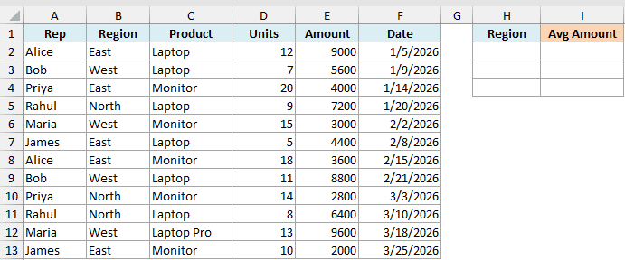
First, enter =UNIQUE(B2:B13) in H2 to list the regions. Then enter this formula in I2 to calculate their averages:
=AVERAGEIFS(E2:E13, B2:B13, UNIQUE(B2:B13))
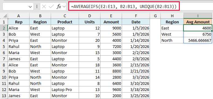
UNIQUE pulls out the distinct regions (East, West, North), and AVERAGEIFS returns one average for each. The result spills down automatically, so East shows 4600, West 6750, and North about 5467. No dragging, no copying the formula down.
This works in Excel 365, Excel 2024, Excel 2021, and Excel for the web. In Excel 2019 and earlier, write a separate AVERAGEIFS for each region instead.
Example 7: Average With OR Criteria (Either Condition)
Now let’s average amounts for either of two regions.
Using the same sales dataset in A1:F13, the regions are in B2:B13 and the amounts are in E2:E13. H2 holds the result label, with I2 empty for now.
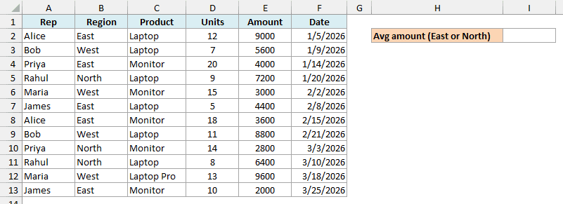
Let’s calculate the average sale amount for East OR North.
Here is the formula:
=SUM(SUMIFS(E2:E13, B2:B13, {"East","North"}))/SUM(COUNTIFS(B2:B13, {"East","North"}))
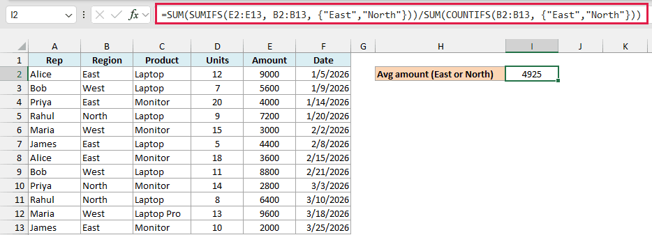
This returns 4925 in I2, the average across all eight East and North rows.
How this formula works:
- SUMIFS returns the two region totals, 23000 and 16400. The outer SUM adds them to get 39400.
- COUNTIFS returns the two row counts, 5 and 3. SUM adds them to get 8.
Dividing 39400 by 8 gives us 4925. To include more regions, add them inside the braces in both places.
AVERAGEIFS joins its criteria with AND. Asking for “East” and “North” as separate criteria on the same Region column requires each row to match both, so nothing matches and it returns #DIV/0!.
Averaging the two region averages gives the wrong result:
=AVERAGE(AVERAGEIFS(E2:E13, B2:B13, {"East","North"}))
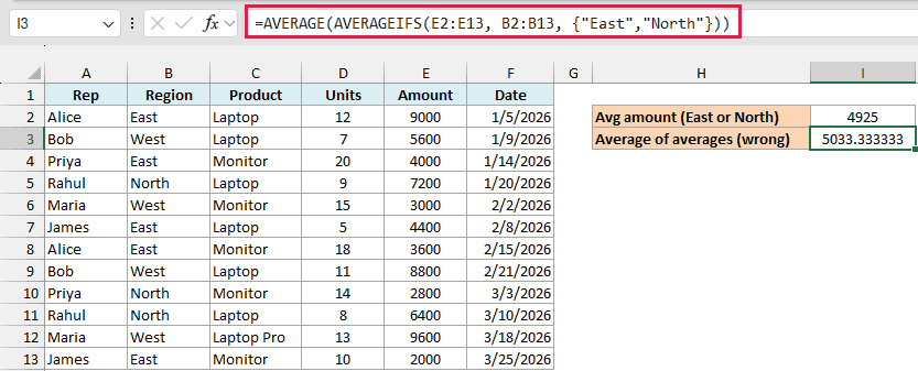
This returns about 5033.33 in I3 (displayed as 5033.333333), while I2 still shows 4925. It averages East’s 4600 and North’s 5466.67.
North’s three rows get the same weight as East’s five rows. Adding the amounts and dividing by the total row count gives every row the same weight.
AVERAGEIF vs AVERAGEIFS
These two look almost identical, and the extra “S” is easy to miss. The difference is simple:
- AVERAGEIF handles a single condition. Its order is
=AVERAGEIF(range, criteria, [average_range]), with the range you average last (and optional). - AVERAGEIFS handles one or more conditions. Its order is
=AVERAGEIFS(average_range, criteria_range1, criteria1, ...), with the range you average first.
If you only ever have one condition, either one works. The moment you need a second condition, reach for AVERAGEIFS.
My habit is to just use AVERAGEIFS everywhere. The argument order is always the same, so I never have to remember which version I’m in.
Things to Keep in Mind
A few points that save headaches when working with AVERAGEIFS:
- average_range goes first. Unlike AVERAGEIF, the range you’re averaging is the first argument, not the last.
- Ranges must match in size. average_range and every criteria_range must cover the same number of rows, or Excel returns a #VALUE! error.
- Quote your operators and text. Conditions like “>100”, “<>East”, or “Laptop” go in double quotes. Bare numbers don’t.
- Blank cells depend on the criterion. In criteria ranges,
0and"<6"skip blanks, while"<>5"includes them. Use""for blanks and"<>"for non-blank cells. - Every criterion must be true. AVERAGEIFS uses AND logic. A row is included only when it satisfies all the conditions at once. Example 7 shows how to handle OR logic.
That covers the main ways to use AVERAGEIFS in Excel, from two simple criteria to date ranges, wildcards, OR logic, and a modern per-category spill.
Once you’re comfortable with the average_range-first order, it works just like SUMIFS and COUNTIFS. I hope you found this tutorial helpful.
Other Excel Articles You May Also Like:
- How to Use Excel AVERAGE Function
- How to Use Excel SUM Function
- How to Use Excel SUMIF Function
- How to Use Excel SUMPRODUCT Function
- Calculating Weighted Average in Excel
- How to Calculate Average Annual Growth Rate (AAGR) in Excel
- SUMIF vs SUMIFS in Excel: What’s the Difference?
- MAXIFS Function in Excel
