

ISNONTEXT checks whether a value is anything other than text. It returns TRUE for numbers, dates, logical values, errors, and empty cells, and FALSE for text.
That last detail can be easy to miss: an empty cell counts as non-text, but a formula that returns an empty string doesn’t. Two cells can look blank and give different results.
In this tutorial, I’ll show you how to check a range, understand those blank-looking cells, flag entries for review, and count non-text values.
Follow along with the example file
ISNONTEXT Function Examples.xlsx
ISNONTEXT Function Syntax
Here is the syntax of the ISNONTEXT function:
=ISNONTEXT(value)
- value – The value you want to test. This required argument can be a cell reference, a value entered directly, or a formula whose result you want to check.
You can also supply a range in Excel versions that support dynamic arrays. This checks each cell and returns a separate result for it.
ISNONTEXT works in Excel 365, 2024, 2021, 2019, 2016, Mac, and the web. The spilling examples below need Excel 365, 2024, 2021, or the web.
When to Use the ISNONTEXT Function
Use this function when you need to:
- Separate text entries from other types of values in a mixed column.
- Check why two cells that look empty give different results.
- Flag non-text entries in a column meant to hold text.
- Count all non-text cells in a range, including empty cells.
Let’s start with a simple TRUE or FALSE check.
Example 1: Check a Range for Non-Text Values
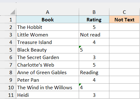
Below is a book-rating list with numbers and text entries, and I want column C to show which ratings are not text.
Enter this formula in cell C2:
=ISNONTEXT(B2:B11)
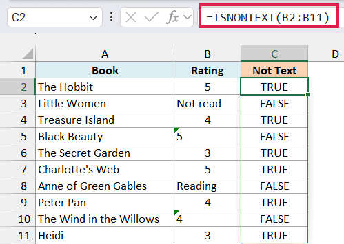
The formula checks each rating and spills ten results down column C. TRUE means the corresponding rating is not text, while FALSE means it is text.
The rating for The Hobbit is the number 5, so it returns TRUE. Black Beauty also shows 5, but that value is stored as text, so it returns FALSE.
ISNONTEXT tests the stored value without converting it. That’s why both the notes, such as “Not read”, and the numbers stored as text return FALSE.
Keep the cells below C2 empty before entering the formula so Excel has room for the results. An occupied cell in the output range can cause a #SPILL! error.
If you’re using Excel 2019 or earlier, enter the following formula in C2 and copy it down to C11:
=ISNONTEXT(B2)
Example 2: Test Blank Cells and Empty Strings
Now let’s look at the inputs that can make this test confusing.
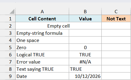
Below is a list of different cell contents, and I want column C to show whether each value is non-text.
Enter this formula in C2:
=ISNONTEXT(B2:B9)
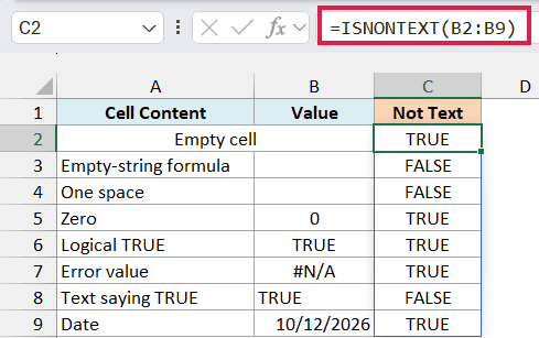
B2 is genuinely empty, so its result is TRUE. B3 contains a formula returning an empty string, so its result is FALSE even though the cell looks empty.
B4 contains one space, which is also text. A space isn’t the same as an empty cell, so this row returns FALSE too.
The two TRUE entries in column B also have different results. B6 contains the logical value TRUE and returns TRUE, while B8 contains the text “TRUE” and returns FALSE.
Zero, the #N/A error, and the date all return TRUE because none is text. Excel stores a real date as a number, and ISNONTEXT can test an error value without passing that error through to its result.
Important: TRUE from ISNONTEXT can mean a number, an empty cell, a logical value, or an error. Use the ISNUMBER function when you need to test specifically for numbers.
In Excel 2019 or earlier, enter this formula in C2 and copy it down to C9:
=ISNONTEXT(B2)
Example 3: Flag Non-Text Entries with IF
TRUE and FALSE work well for a quick check, but a label can make the result easier to act on.
Below is a trip list where the destination should be text, and I want column C to flag non-text entries for review.
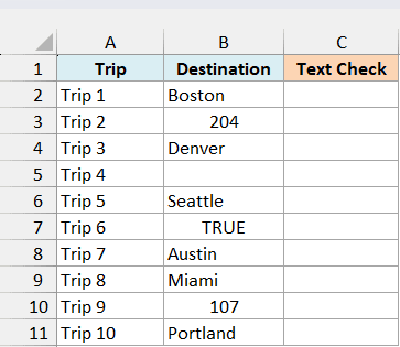
Enter this formula in C2:
=IF(ISNONTEXT(B2:B11),"Review","Text")
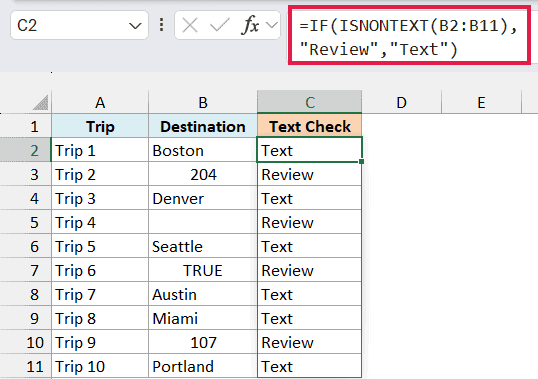
ISNONTEXT checks each destination first. The IF function returns “Review” when that check is TRUE and “Text” when it is FALSE.
Trips 2, 4, 6, and 9 are marked for review because their destination cells contain 204, an empty cell, TRUE, and 107. The remaining entries contain text.
The label “Text” only describes the value’s type. It doesn’t confirm that a city name is correct, and it would also accept a space or a number stored as text.
If you’re using Excel 2019 or earlier, enter this single-cell version in C2 and copy it down to C11:
=IF(ISNONTEXT(B2),"Review","Text")
Example 4: Count Non-Text Cells
You can also count the non-text entries without adding a result beside every row.
Below is a delivery-note list, and I want cell D2 to show how many note cells contain something other than text or are empty.
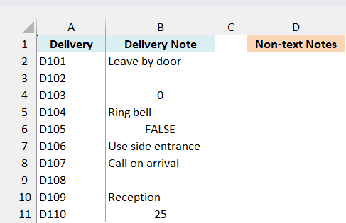
Enter this formula in D2:
=SUMPRODUCT(--ISNONTEXT(B2:B11))
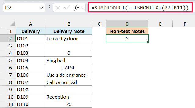
The result is 5. That includes the two empty note cells, the numbers 0 and 25, and the logical value FALSE.
How this formula works:
ISNONTEXT(B2:B11)returns TRUE for each non-text cell and FALSE for each text cell.- The double minus (
--) converts those TRUE and FALSE results into 1s and 0s. - The SUMPRODUCT function adds the 1s and 0s to give the total number of non-text cells.
The SUM function can also add this array in modern Excel. This example uses the SUMPRODUCT function so the same formula works in Excel 2019 and earlier with a normal Enter, without special array entry.
Important: Empty cells count toward this total. Use the actual data range rather than a whole-column reference, or the unused empty cells will inflate the result.
In this tutorial, I showed you how to use ISNONTEXT to check cell values, flag entries with IF, and count non-text cells. Remember that empty cells and errors count as non-text too.
I hope you found this article helpful.
Other Excel Articles You May Also Like:
